BRAIN SPEC Lab · NC State

Research

Understanding how processors behave—and making them more secure, efficient, and explainable.

The privacy cost of efficient AI

Power gating and sparsity make AI faster and more energy efficient. Our work asks what those optimizations reveal about the computation—and how to close the resulting channels.

TranScope

Hardware footprints reveal what model outputs can hide.

TranScope examines how tokenization and embedding access patterns affect caches, TLBs, and on-core accelerators during inference. With local control of the hardware, operating system, and runtime, an auditor measures these footprints to distinguish input distributions associated with training data.

Key findingLocal hardware evidence

The study evaluates distributional inference through privileged hardware measurements.

Paper · PDFarXiv recordBibTeX

Significant findings

98% reported accuracy

Distributional information in hardware footprints

The abstract reports 98% out-of-distribution detection accuracy, with 1.5% false positives and 2.5% false negatives, for the evaluated large-scale model setting.

0.9 reported AUC

Stronger separation in the reported comparison

The abstract reports 0.9 AUC for TranScope versus 0.6 for PETAL. This is evidence from the paper’s evaluated setting, not a universal accuracy guarantee.

Cache + TLB locality

A mechanism behind the signal

Tokenization and embedding access patterns can change token locality, TLB behavior, and page-table walks even when software paths are alike.

Beyond output scores

Confidence hiding leaves hardware signals

The evaluated output-discretization defenses do not remove TranScope’s signal. Measurements require a local auditor with control of hardware, OS, and inference runtime; distributional inference alone does not establish exact training-record membership.

Explore the evidence

9 figures · Select a preview to enlarge
Figure 1

Hardware inference under confidence-hiding defenses
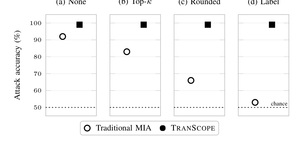
Hardware inference under confidence-hiding defenses. The evaluated hardware classifier is compared with a software baseline under different restrictions on model outputs.

The evaluated hardware classifier is compared with a software baseline under different restrictions on model outputs.

Figure 2

Classification accuracy as models scale
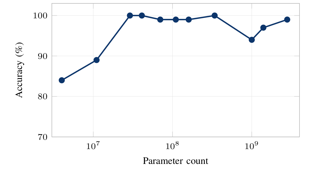
Classification accuracy as models scale. Each point reports the highest accuracy at that model scale across the evaluated families.

Each point reports the highest accuracy at that model scale across the evaluated families.

Figure 3

Socket-power footprints across model sizes
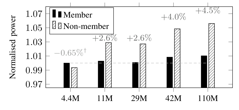
Socket-power footprints across model sizes. The plot compares normalized per-inference socket-power measurements for the evaluated input groups.

The plot compares normalized per-inference socket-power measurements for the evaluated input groups.

Figure 4

From token locality to memory-hierarchy behavior
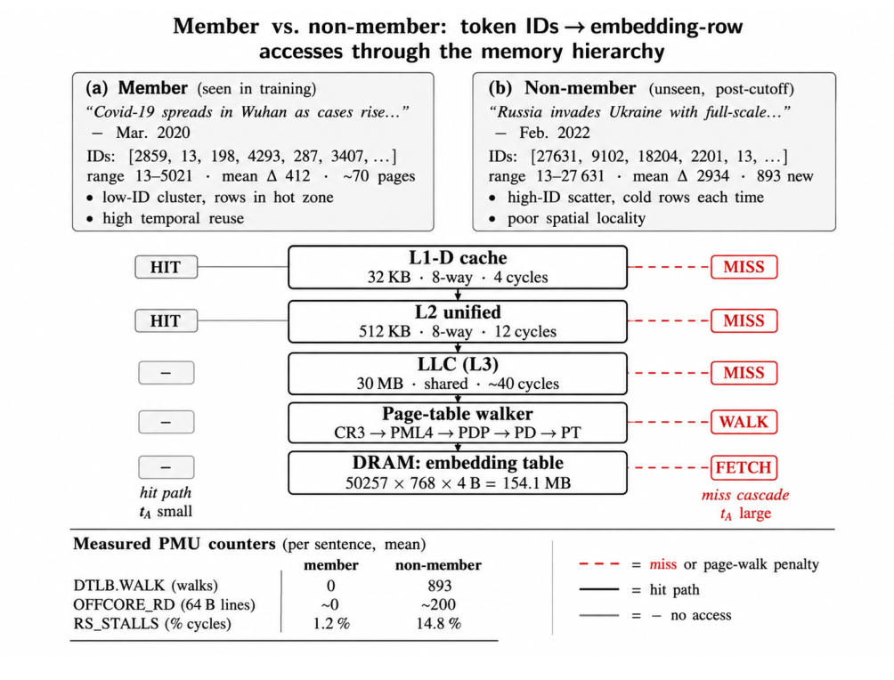
From token locality to memory-hierarchy behavior. The mechanism diagram traces clustered and scattered embedding accesses through caches, TLBs, and page-table walks.

The mechanism diagram traces clustered and scattered embedding accesses through caches, TLBs, and page-table walks.

Figure 5

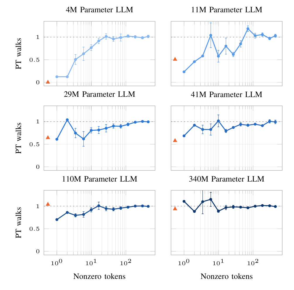
Page-table walks and token structure

Page-table walks and token structure. The experiments vary zero-token counts and model size to examine their effects on page-table walks.

The experiments vary zero-token counts and model size to examine their effects on page-table walks.

Figure 6

Token-distance distributions across model sizes
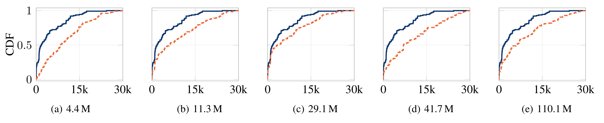
Token-distance distributions across model sizes. The distributions compare successive token distances for in-distribution and out-of-distribution samples.

The distributions compare successive token distances for in-distribution and out-of-distribution samples.

Figure 7

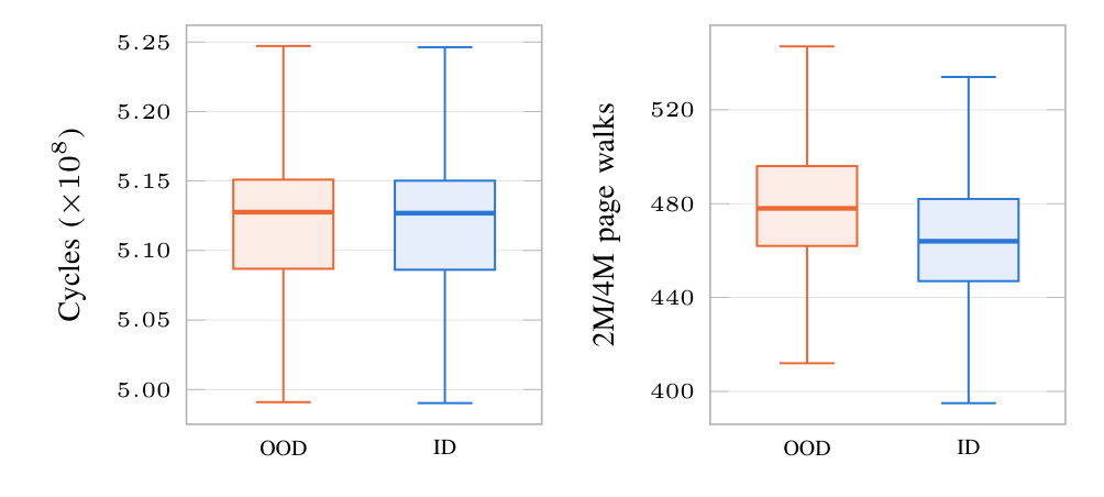
Cycle counts and page-table walks

Cycle counts and page-table walks. The evaluated input groups can have similar inference cycle counts while producing different page-table-walk footprints.

The evaluated input groups can have similar inference cycle counts while producing different page-table-walk footprints.

Figure 8

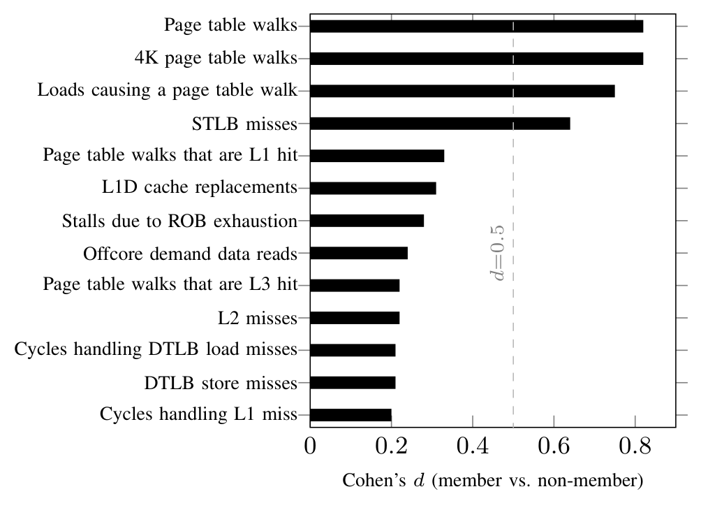
Counter signals on Haswell

Counter signals on Haswell. The figure ranks the evaluated BERT-tiny hardware-counter signals by effect size.

The figure ranks the evaluated BERT-tiny hardware-counter signals by effect size.

Figure 9

Counter signals in a Vision Transformer
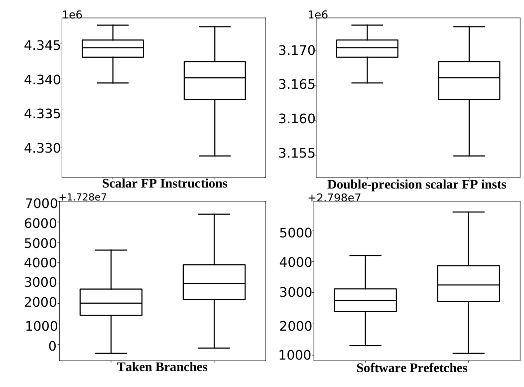
Counter signals in a Vision Transformer. Four measured counters illustrate hardware-footprint differences for the evaluated Vision Transformer inputs.
Four measured counters illustrate hardware-footprint differences for the evaluated Vision Transformer inputs.
GateBleed

An accelerator’s wake-up time reveals more than its power state.

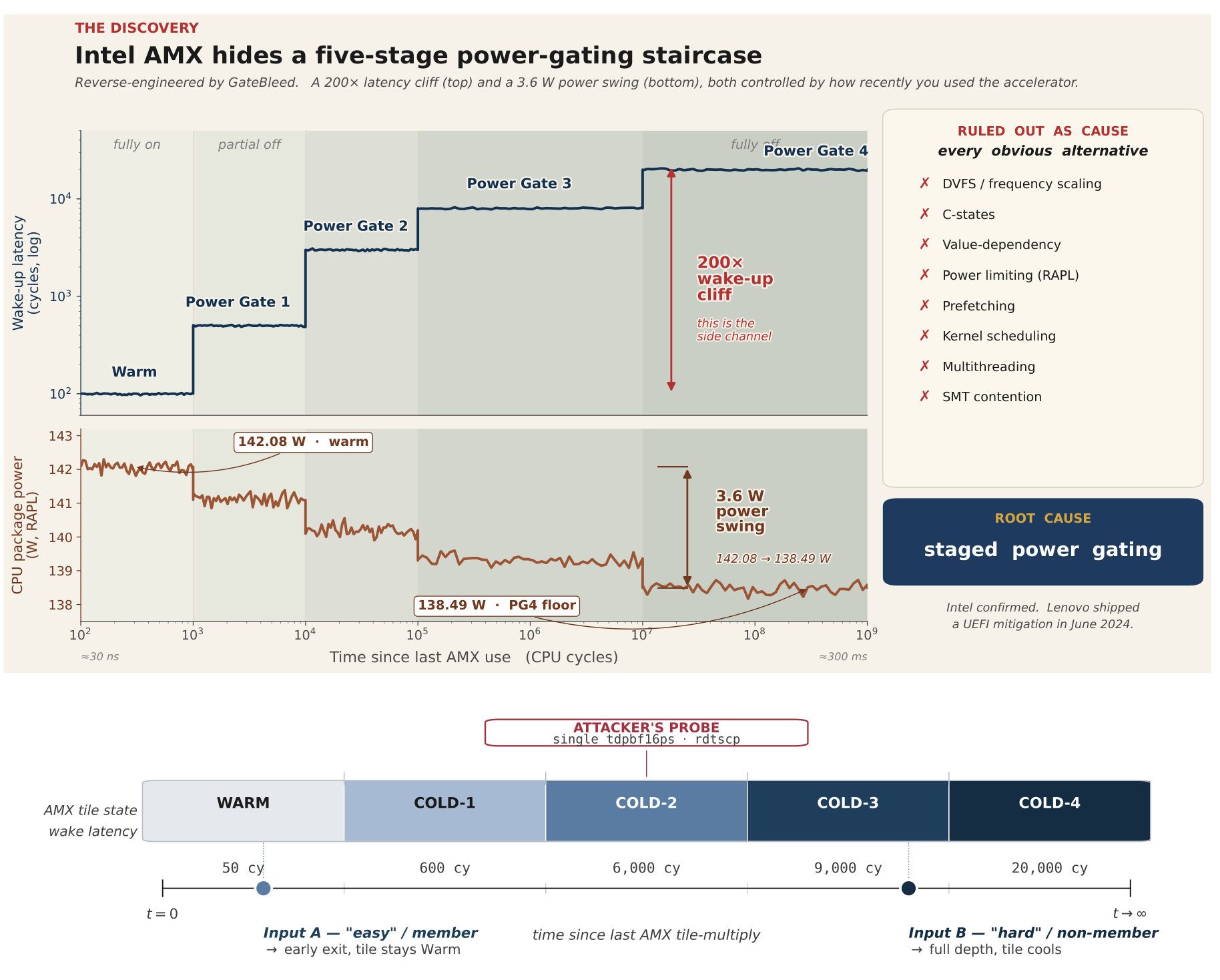
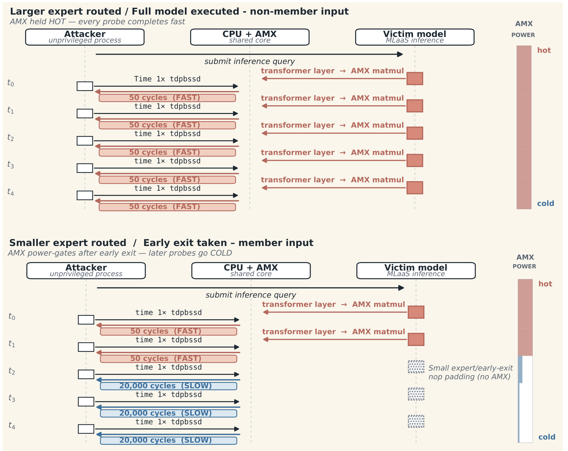
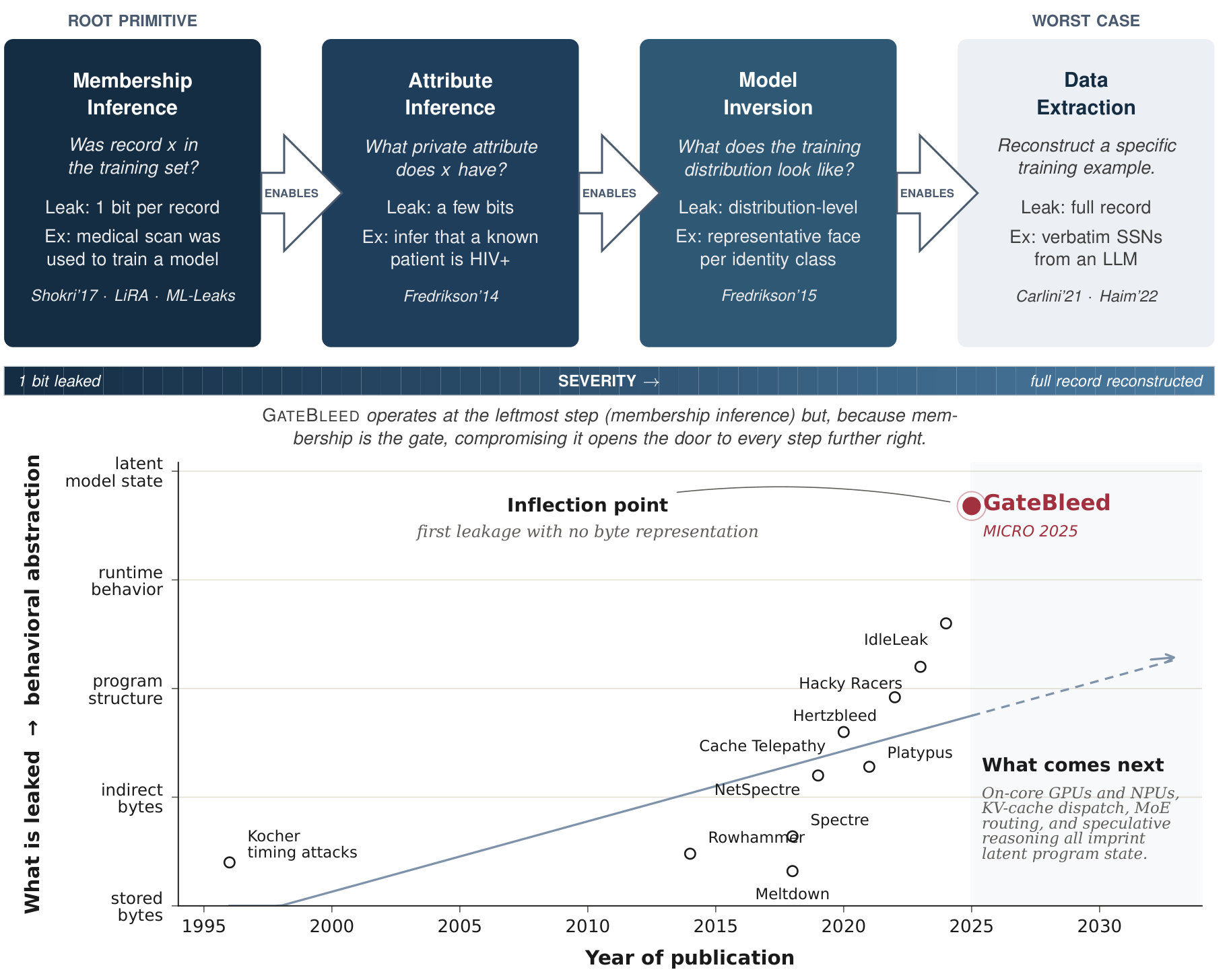
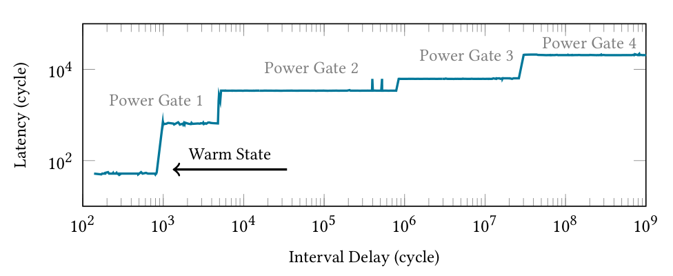
Intel AMX enters progressively deeper sleep states between uses. Timing its next operation reveals how recently another computation used the accelerator. GateBleed turns that signal into information about AI execution and training-data membership, without reading the model’s confidence scores.

Key finding99%

Membership-inference accuracy on the evaluated early-exit CNN; 81% on the evaluated Transformer.

Paper · PDFSlidesPoster · PDFCodeBibTeX
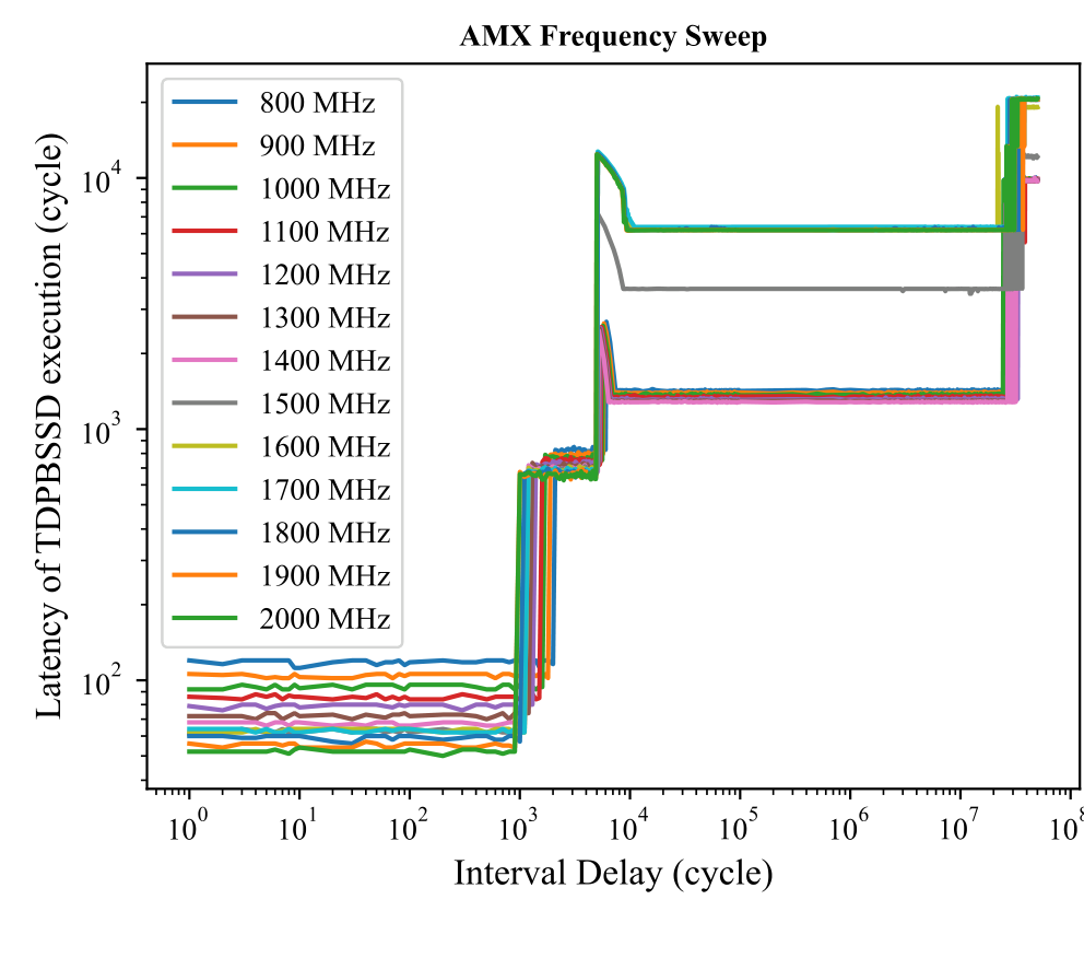
AMX latency increases in steps as the idle interval grows, from a warm state through four power-gated states.

The latency staircase makes AMX’s hidden power states observable. Longer idle intervals lead to more expensive wake-ups.

Figure 1 · MICRO 2025Full-size figureSource page

Explore the evidence

7 figures · Select a preview to enlarge
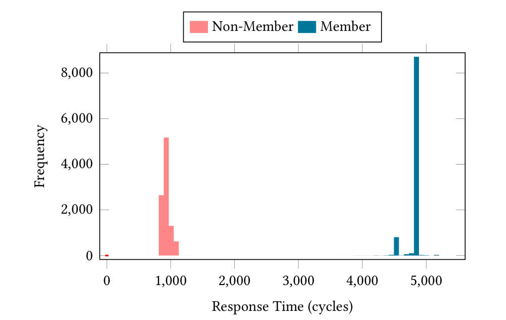
Figure 3

Training-member and non-member timing distributions

Two response-time histograms after CNN inference: non-member measurements cluster near 1,000 cycles, while member measurements cluster near 4,700 cycles.

After CNN inference, the measured AMX response-time distributions separate training-set members from non-members in the reported experiment.

Figure 4

Leakage signal across fixed core frequencies

AMX execution latency plotted against interval delay across fixed CPU frequencies, showing similar stepwise power-gating latency states.

The timing stages remain visible across the fixed core frequencies evaluated in the paper.

Figure 7

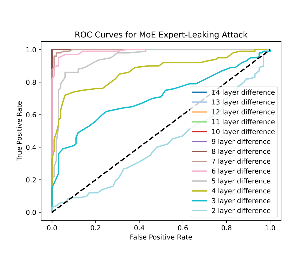
Expert-routing inference across layer differences

ROC curves for GateBleed expert-routing inference at layer-count differences from two to fourteen layers; larger differences produce stronger true-positive and false-positive separation.

ROC curves compare GateBleed’s expert-leakage accuracy as the two experts’ layer counts diverge. The plotted separation depends on the evaluated model configuration.

Figure 8

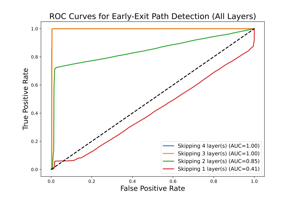
Early-exit inference across exit depths

ROC curves for CNN membership inference with one to four layers skipped; curves differ in true-positive rate as false-positive rate increases.

The ROC curves show the membership signal for early exits at different network depths in the evaluated CNN.

Figure 9

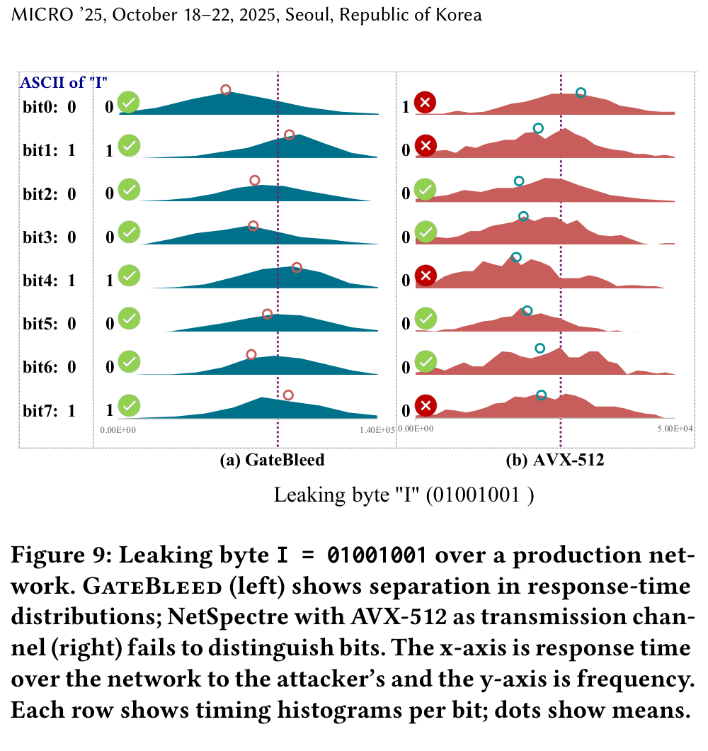
A timing signal carries across a production network

Eight timing distributions show GateBleed recovering the byte 01001001 over a production network, while the comparison channel misses several bits.
The byte-recovery experiment compares GateBleed with a conventional network timing channel across eight bit positions.
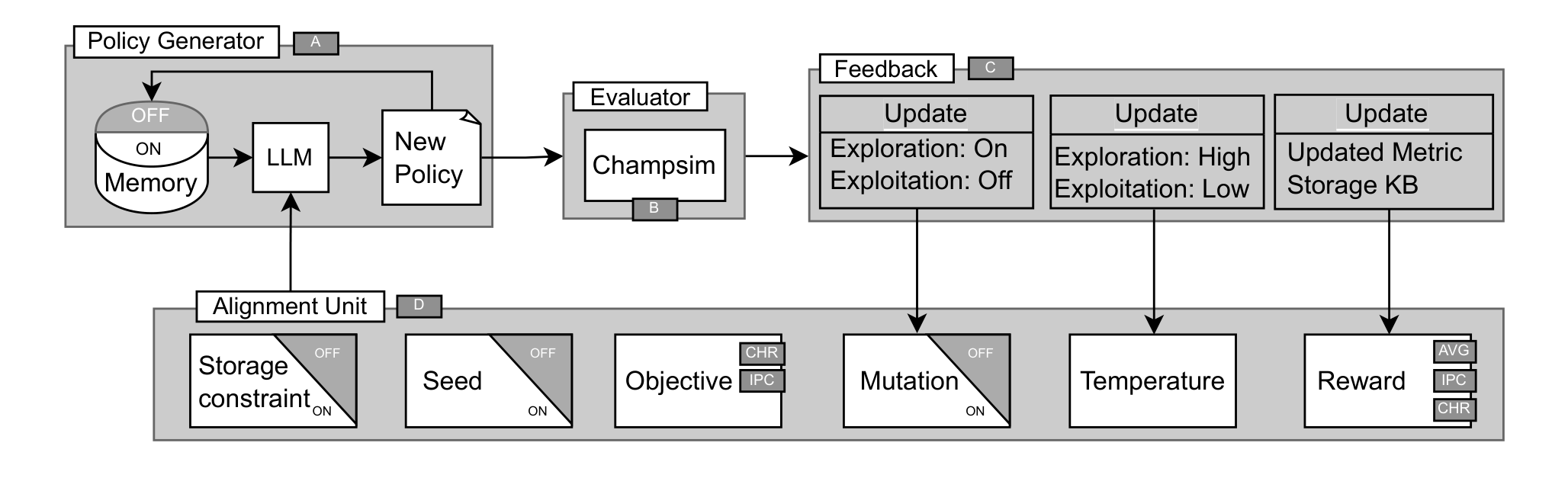
Figure 10

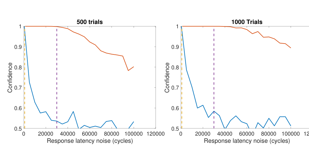
Network-noise resilience at two trial counts

Two line charts show confidence against injected network noise for GateBleed, AVX-512, and the local-noise baseline, at 500 trials and 1,000 trials.
At 500 and 1,000 trials, the plot compares GateBleed’s measured confidence with AVX-512 and the local network-noise baseline. Results apply to the paper’s evaluated network setting.

Figure 12

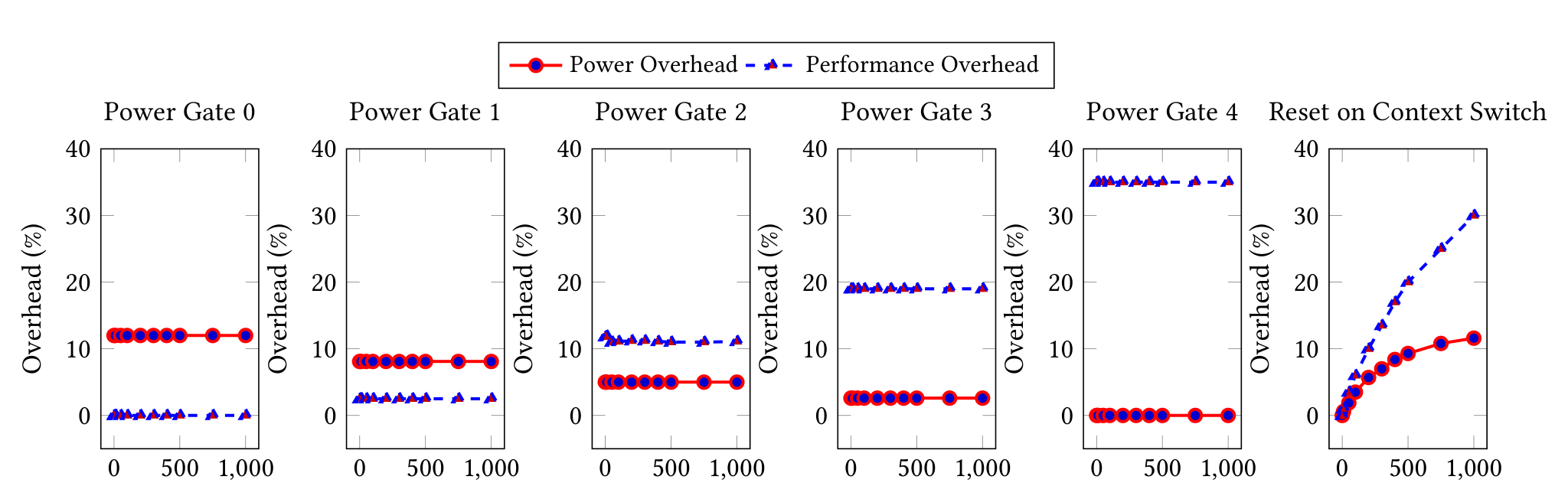
Power and performance costs of mitigation

Six small line charts compare power overhead and performance overhead across context-switch rates for AMX power-gating states zero through four and reset on context switch.

Six panels compare power and performance overhead as context-switch rate increases, for several AMX power-gating states and reset-on-switch.

FeatureBleed

Faster inference can reveal private features behind an API.

A prediction service may enrich a request with private records that the caller never sees. FeatureBleed shows how skipping zero-valued computations can make those hidden features distinguishable through end-to-end inference time. The study spans medical and socioeconomic data and evaluates a timing-padding defense.

Key finding3 hardware backends

Evaluated on Intel AVX, Intel AMX, and NVIDIA A100 across three model architectures.

Paper · PDFBibTeX
Inference-time distributions for six medical attributes have distinct peaks, showing a timing channel.

Distinct timing distributions expose differences between private medical attributes in the paper’s evaluated workload.

Figure 1 · IEEE CAL 2026Full-size figureSource page

Explore the evidence

1 figures · Select a preview to enlarge
Figure 3

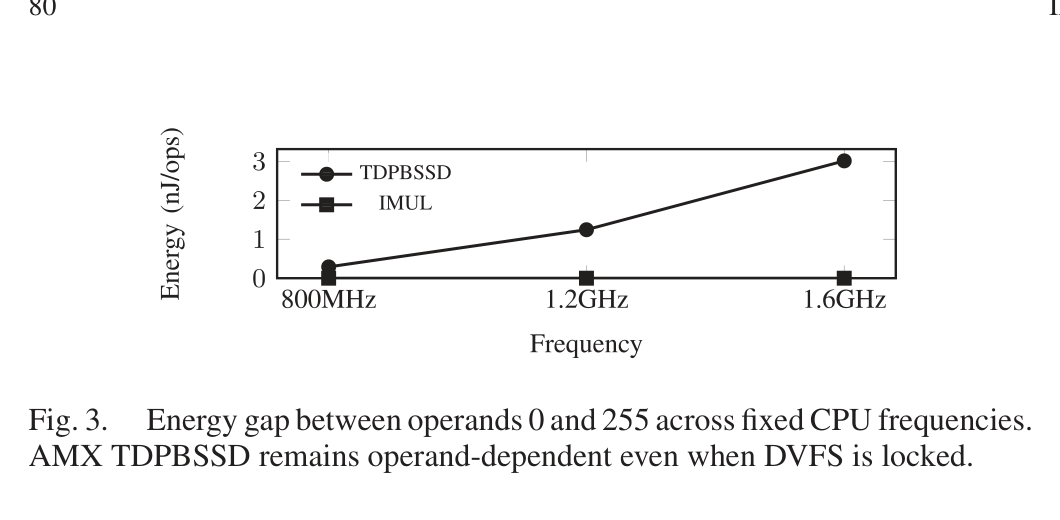
The operand timing gap persists across CPU frequencies

A line chart compares energy for two AMX operands at 800 megahertz, 1.2 gigahertz, and 1.6 gigahertz; the gap grows with frequency.

The energy gap between operands 0 and 255 remains visible at fixed frequencies in the reported AMX experiment.

THOR

Even non-speculative matrix operations can leak model structure.

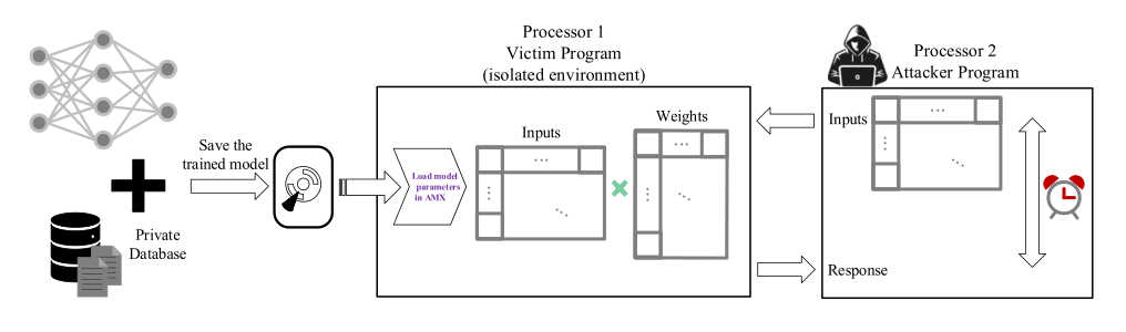
THOR studies a value-dependent timing channel in Intel AMX. Carefully chosen inputs let an unprivileged attacker infer whether neural-network weights are zero or nonzero, without physical access or model confidence scores. The work also measures the power cost of its proposed countermeasure.

Key finding64 weights

Their zero/nonzero pattern was recovered within 50 minutes in the reported experiment.

Paper · PDFBibTeX
THOR threat model: a victim processes inputs using private neural-network weights while an attacker observes response timing.

The threat model connects private model weights to timing measurements made by an attacker-controlled program.

Figure 1 · IEEE CAL 2025Full-size figureSource page

Explore the evidence

1 figures · Select a preview to enlarge
Figure 2

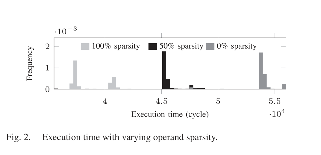
Execution time changes with operand sparsity

A frequency plot shows distinct AMX execution-time clusters for inputs with 100 percent, 50 percent, and zero percent sparsity.

The measured AMX execution-time distributions separate inputs with different operand sparsity in this workload.

Exploiting Intel AMX Power Gating

A local power optimization becomes a remote transmission channel.

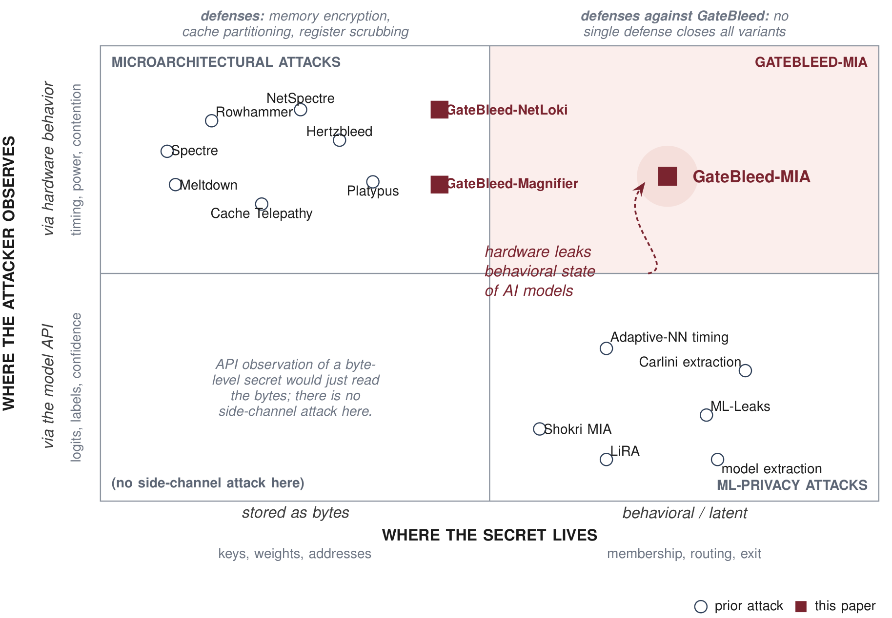
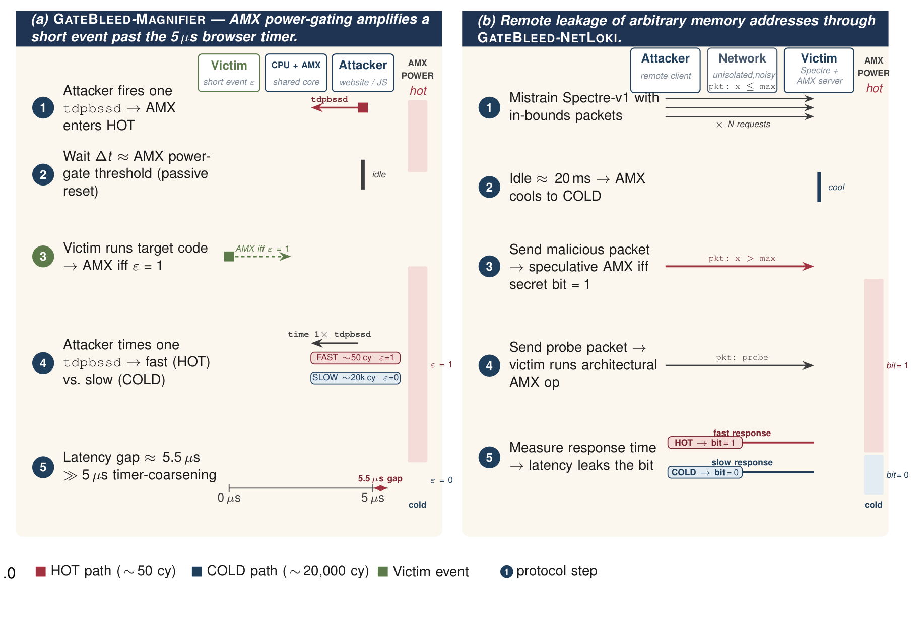
NETLOKI combines speculative execution with AMX power-gating latency to transmit secret bits over a network. In the evaluated network, its timing signal remains distinguishable where the comparison NetSpectre channel fails. This early study establishes the channel and examines a defense that keeps AMX warm.

Key findingBeyond the cache

The transmission signal comes from accelerator power state rather than cache state.

Paper · PDFBibTeX
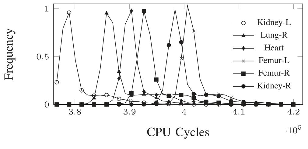
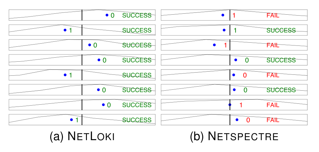
Eight bit measurements recover the byte 01001001 with NETLOKI; NetSpectre fails to distinguish several of the same bits.
A bit-by-bit comparison shows successful bit separation with NETLOKI and overlapping measurements with the comparison channel.

Figure 3 · IEEE CAL 2025Full-size figureSource page

Explore the evidence

1 figures · Select a preview to enlarge
Figure 4

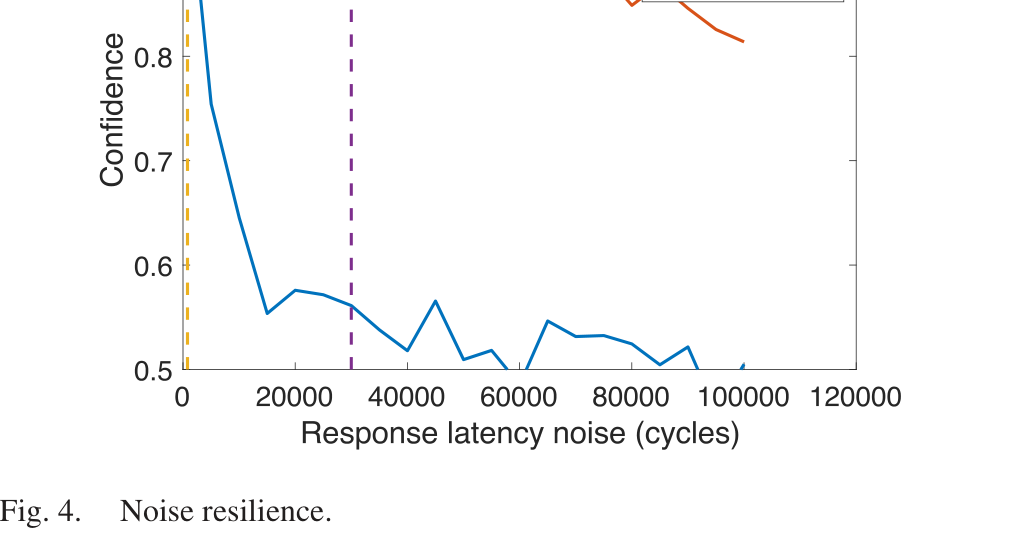
Noise resilience of the network timing signal

A line chart compares confidence for two network timing channels as response-latency noise rises; the proposed channel remains more distinguishable in the evaluated range.

The comparison measures the signal as response-latency noise increases; the result is specific to the evaluated network setting.

GateBleed · IEEE Micro Top Picks

Security, performance, and power must be designed together.

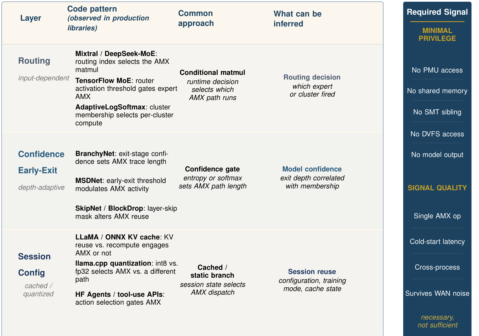
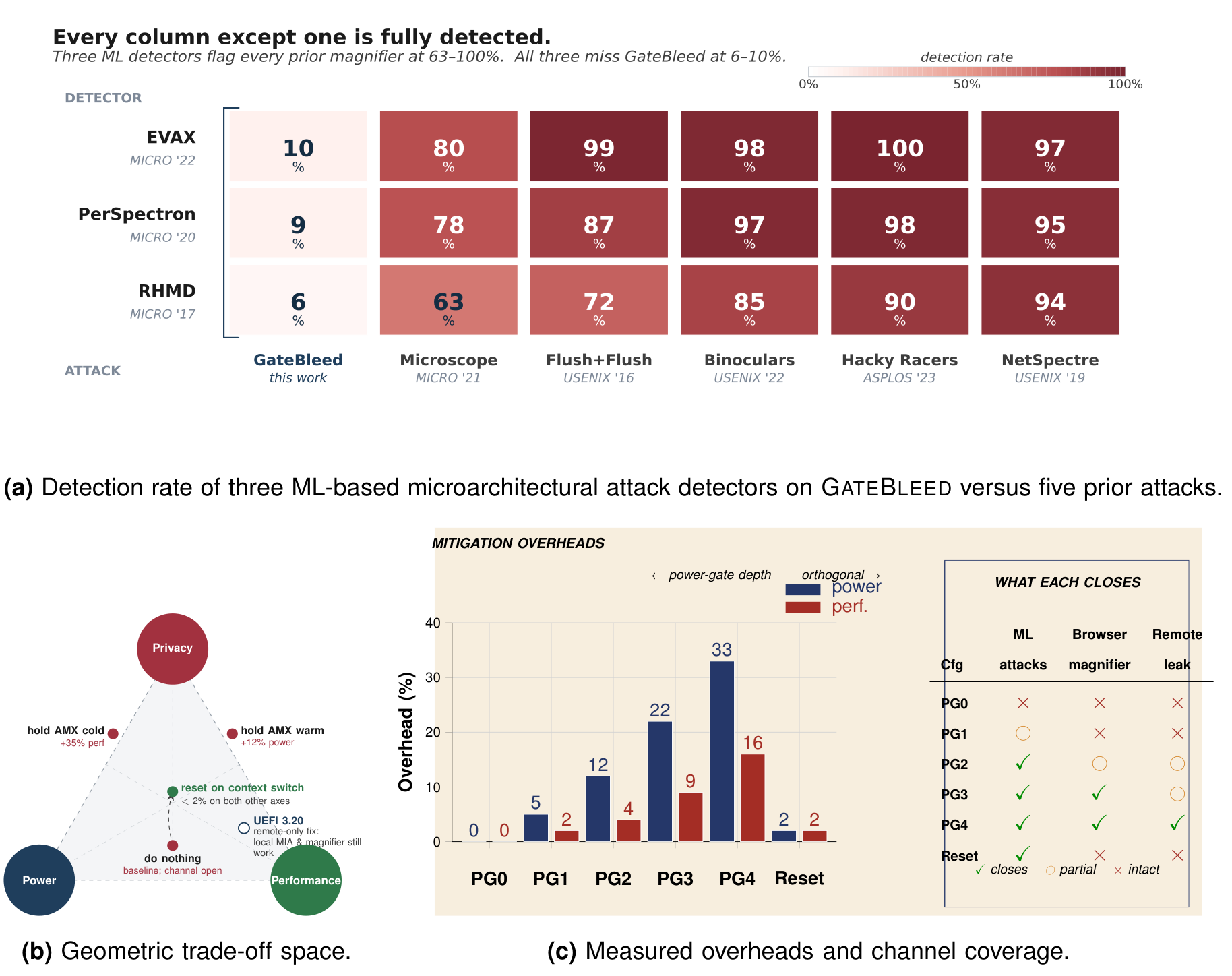
The Top Picks article places GateBleed in the broader design of on-core AI accelerators. It explains why software-level privacy controls do not necessarily close a hardware timing channel, compares detector blind spots, and maps the costs and coverage of proposed mitigations.

Key findingPower · performance · privacy

A three-way design trade-off, examined in the 2026 IEEE Micro Top Picks article.

Paper · PDFBibTeX

Learning to recognize attacks in hardware

Attackers leave patterns in processor activity. We study how lightweight hardware models can recognize those patterns and activate defenses when they are needed.

EVAX

Train for evasive behavior. Apply protection when it matters.

EVAX uses generated attack variations to train detectors and develop security-focused hardware features. The detector controls when a processor enables stronger mitigations. The aim is to retain protection against the evaluated attacks while avoiding the cost of running expensive defenses continuously.

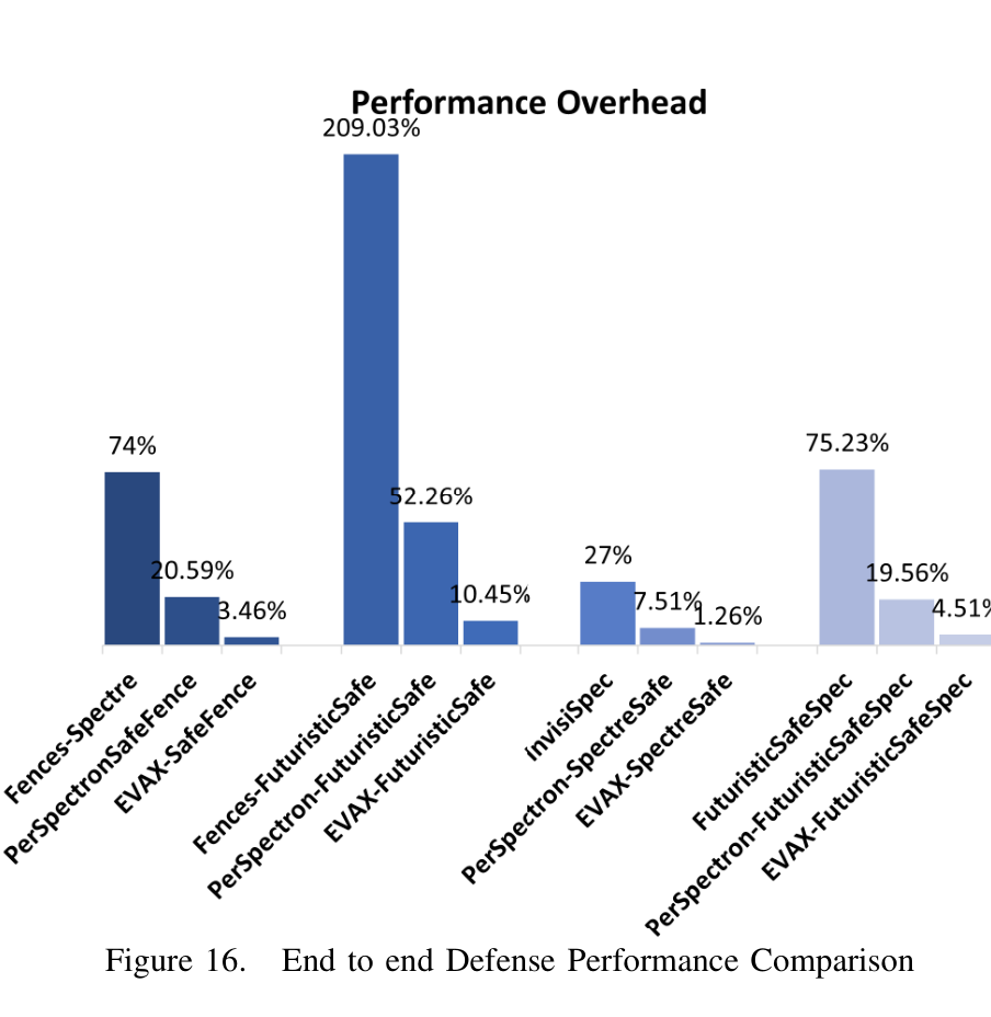
Key finding27% to 1.26%

Reported InvisiSpec performance overhead with EVAX’s adaptive protection in the evaluated workloads.

Paper · PDFSlidesBibTeX
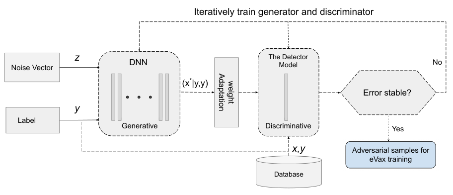
EVAX training loop joins a generative neural network, a detector, iterative weight updates, and a database of adversarial samples.

A generator and detector are trained together to produce adversarial examples for EVAX training.

Figure 3 · MICRO 2022Full-size figureSource page

Explore the evidence

5 figures · Select a preview to enlarge
Figure 13

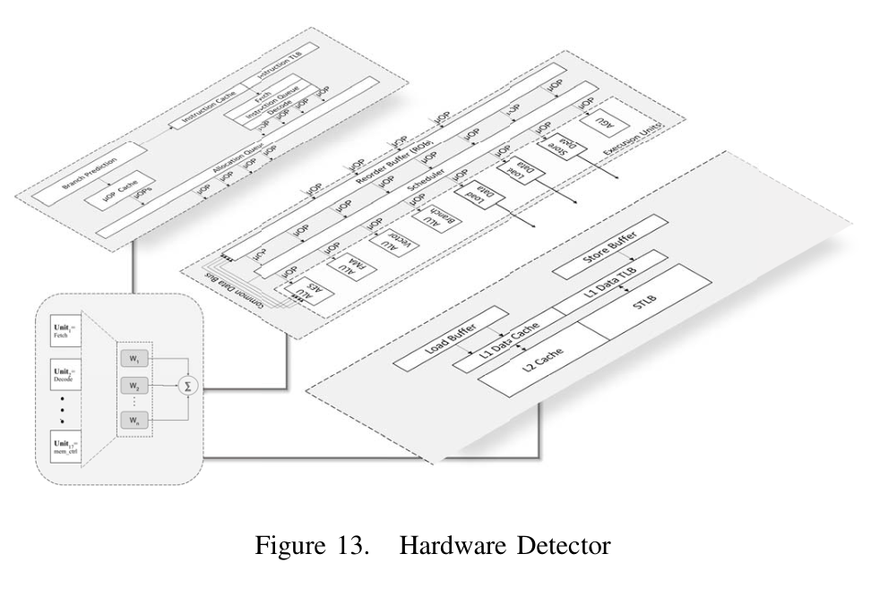
EVAX hardware detector architecture

EVAX hardware detector diagram: processor signals feed a perceptron classifier built from feature inputs, weights, and a threshold decision.

A hardware-level view of the perceptron detector and its signal path, showing how security features feed a compact on-chip detector.

Figure 14

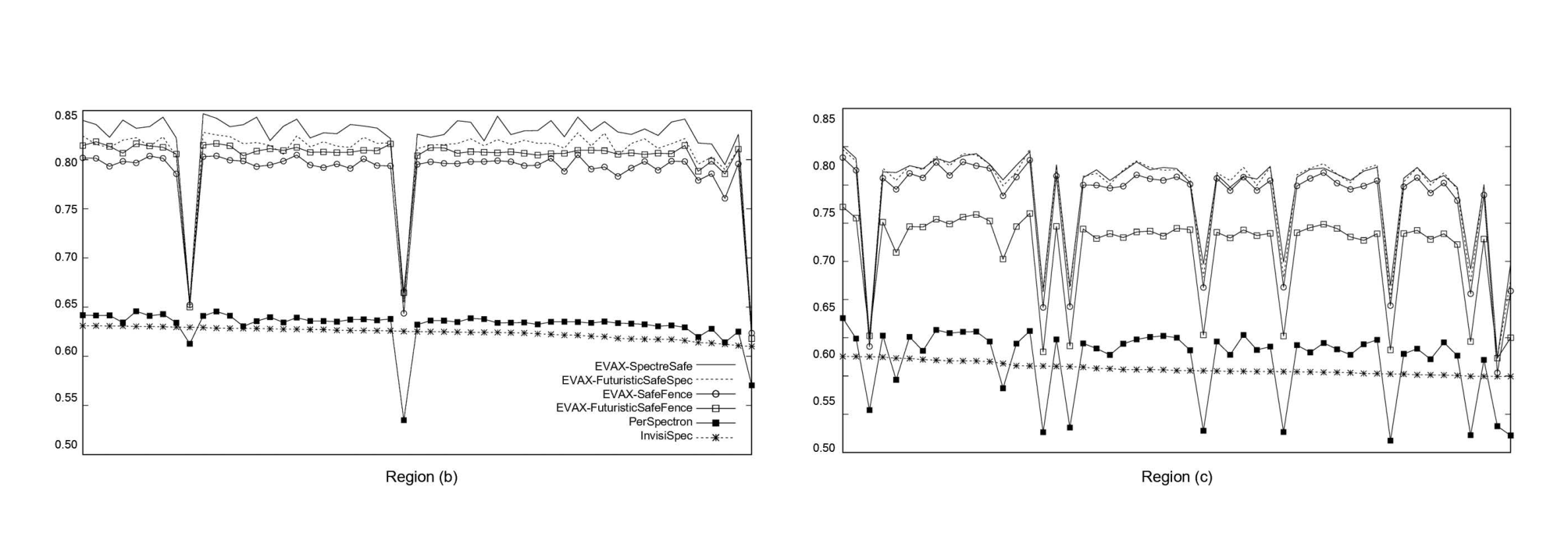
IPC impact of adaptive hardware defenses

Two line plots compare IPC across workload regions for EVAX and other evaluated security defenses, with several sharp workload-dependent drops.

The plots compare instructions per cycle for EVAX, PerSpectron, and InvisiSpec under the evaluated attack-mitigation settings.

Figure 15

False-positive and false-negative distributions

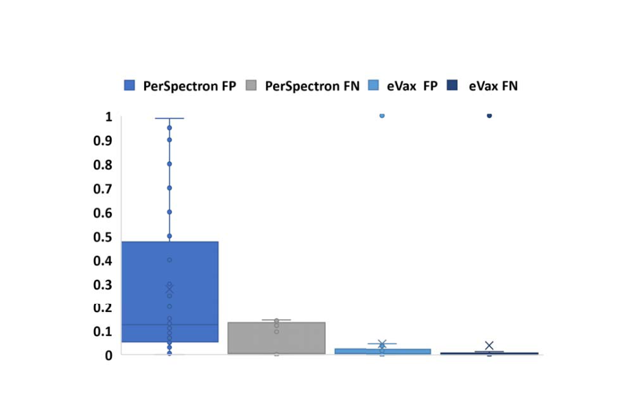
Four bars compare PerSpectron and EVAX false-positive and false-negative rates, with error bars showing the reported distributions.

The comparison summarizes the false-positive and false-negative rates for the evaluated PerSpectron and EVAX detectors.

Figure 16

End-to-end defense performance overhead

Grouped bars compare end-to-end performance overhead for PerSpectron, EVAX, and multiple fence or speculative-execution defense configurations.

The bar chart compares performance overhead for the end-to-end defense configurations evaluated in EVAX.

Figure 17

Detection remains effective against evasive attacks

Two ROC plots compare EVAX and PerSpectron detection for three generated attack families, showing higher true-positive rates as false-positive rates increase.

The ROC curves compare EVAX and PerSpectron detectors against three automatically generated attack families.

PerSpectron

Recognize attack footprints inside the processor.

PerSpectron combines microarchitectural activity from multiple processor components using a small perceptron-based hardware detector. It looks for patterns shared by related attacks, including variants of Spectre, Meltdown, and cache attacks. Detection operates outside the processor’s critical paths.

Key findingEarly detection

The paper reports detection before data leakage for its evaluated attack suite.

Paper · PDFSlidesBibTeX
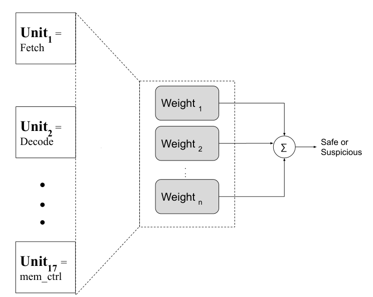
PerSpectron architecture: observations from fetch, decode, memory control and other units feed weighted inputs to a safe-or-suspicious classifier.

Signals from processor units feed learned weights and a compact classifier that distinguishes safe from suspicious activity.

Figure 2 · MICRO 2020Full-size figureSource page

Explore the evidence

1 figures · Select a preview to enlarge
Figure 3

The detector responds to Spectre variants

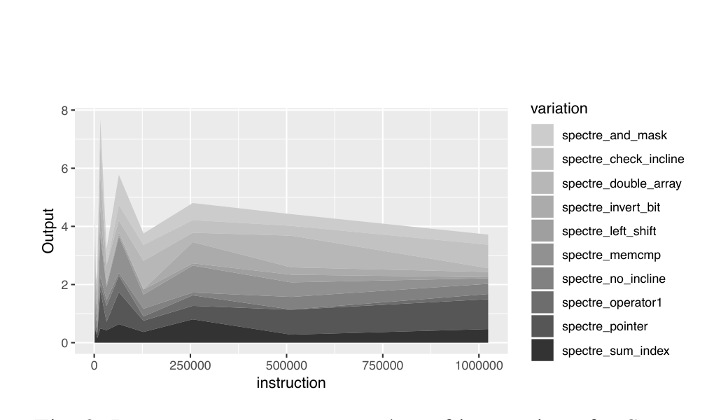
A stacked area plot shows PerSpectron output over one million instructions for several Spectre variations with the same leakage frequency.

The plot tracks PerSpectron’s output as instructions execute for evaluated Spectre variations with the same leakage frequency.

Processors that predict. Tools that explain.

Better decisions about what to fetch, retain, or predict can make limited hardware go further. This work connects compact learning mechanisms with tools for understanding their behavior.

CacheFit

Design the cache policy with its hardware cost in view.

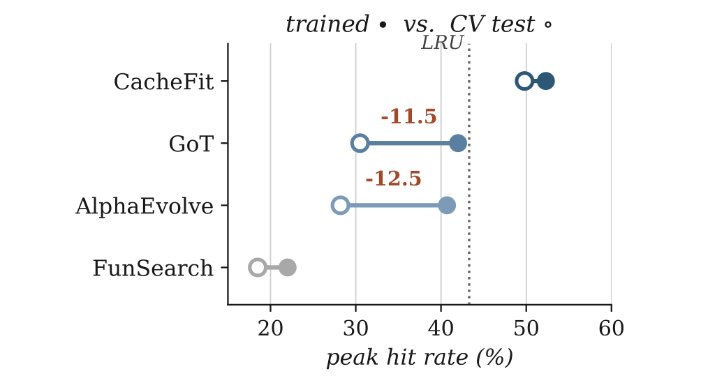
CacheFit uses an LLM to propose and refine last-level cache replacement policies while evaluating performance in ChampSim and hardware cost with HARCOM. Designers set latency, area, and power budgets, and can inspect and edit the search’s recorded proposals and lessons.

Key findingCost inside the search

Performance simulation and analytical hardware-cost modeling guide each redesign.

Paper · PDFarXiv recordBibTeX

Significant findings

60.3% less storage

Fit-MPPPB reduces cost while improving IPC

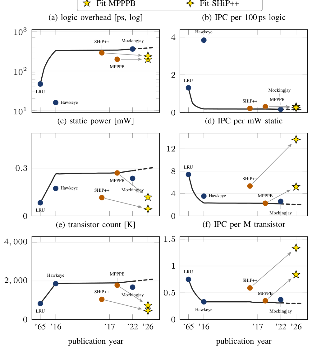
Compared with MPPPB, Fit-MPPPB uses 60.3% less storage, 56.3% less modeled static power, and 58.9% fewer modeled transistors, with 1.1% higher IPC.

61% less static power

Fit-SHiP++ trades a small performance loss for lower cost

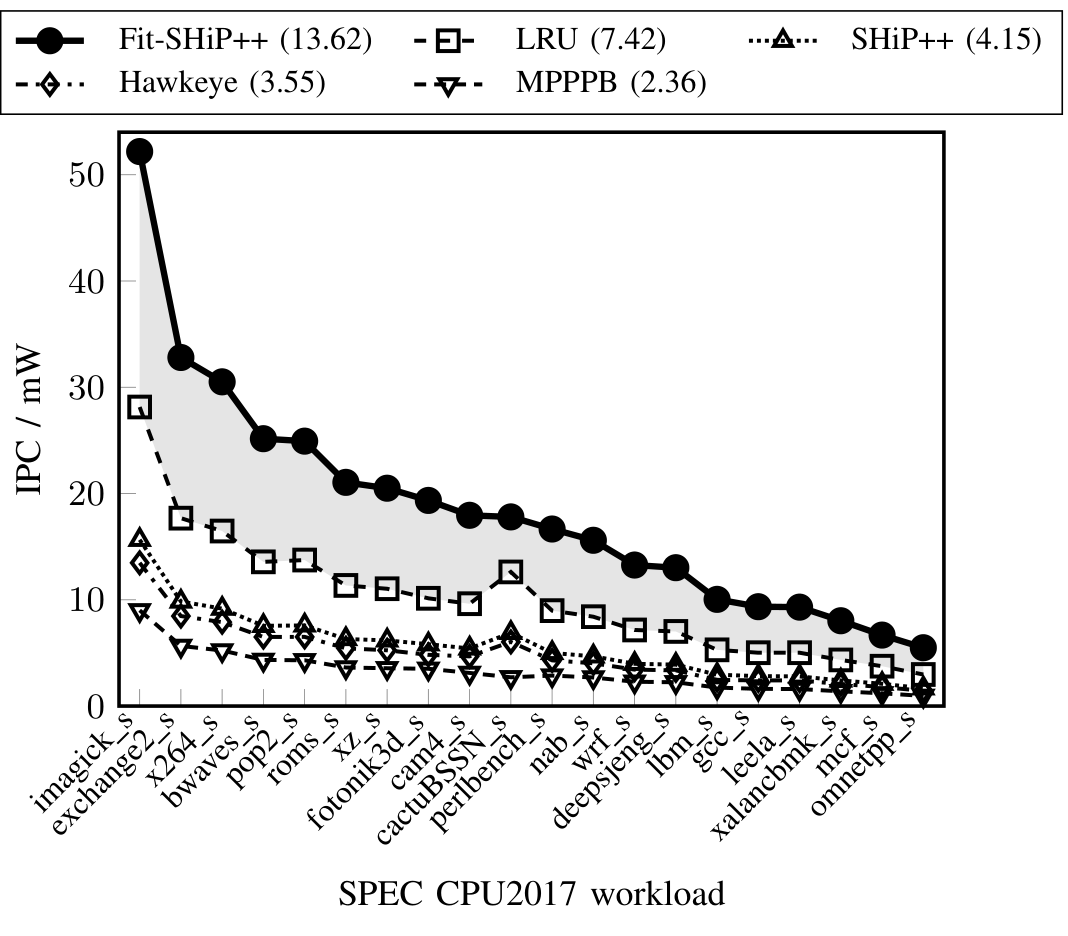
Compared with SHiP++, Fit-SHiP++ reduces modeled static power by 61% and storage by 56%, with 1.54% lower IPC.

Cost from the start

Design decisions account for hardware feasibility

ChampSim measures performance while HARCOM analytically models circuit costs. The designer sets latency, area, and power budgets and can inspect or edit the search memory.

Explore the evidence

8 figures · Select a preview to enlarge
Figure 1

The rising cost of replacement policies

The rising cost of replacement policies. The figure compares hardware costs and performance per unit cost across policies and publication years.

The figure compares hardware costs and performance per unit cost across policies and publication years.

Figure 3

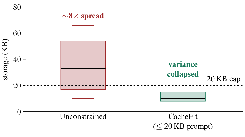
Constraint-driven versus unguided search

Constraint-driven versus unguided search. The comparison shows policy search with and without an explicit 20 KB storage constraint.

The comparison shows policy search with and without an explicit 20 KB storage constraint.

Figure 4

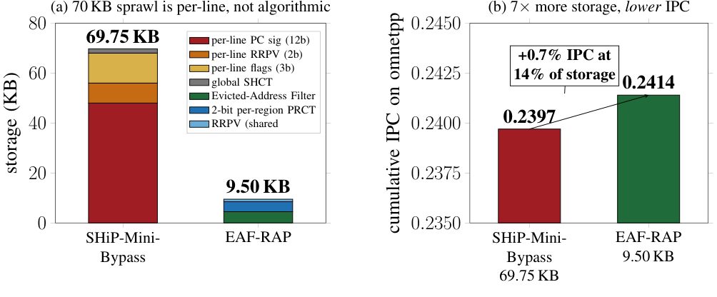
Where a policy spends its storage

Where a policy spends its storage. Two policies from the same unguided search differ in storage allocation and IPC.

Two policies from the same unguided search differ in storage allocation and IPC.

Figure 5

Performance per unit of modeled static power

Performance per unit of modeled static power. Fit-SHiP++ and baselines are compared across 20 SPEC CPU2017 workloads using IPC per modeled milliwatt.

Fit-SHiP++ and baselines are compared across 20 SPEC CPU2017 workloads using IPC per modeled milliwatt.

Figure 6

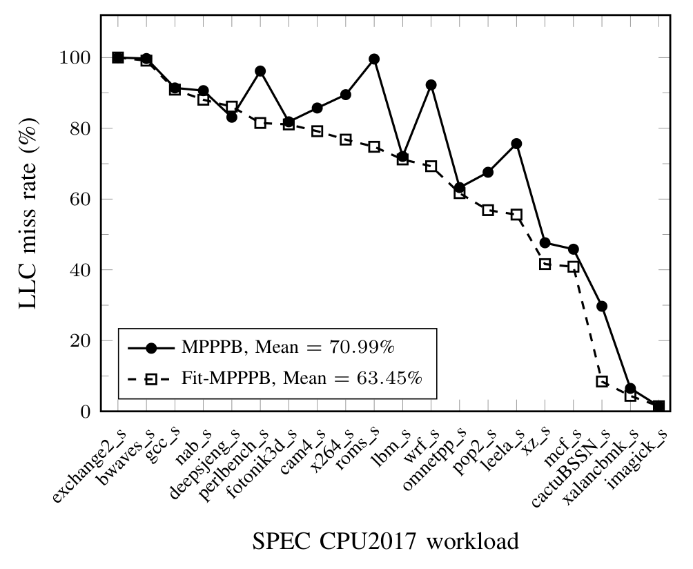
Miss-rate comparison across workloads

Miss-rate comparison across workloads. The plot compares Fit-MPPPB with MPPPB across the evaluated SPEC CPU2017 workloads.

The plot compares Fit-MPPPB with MPPPB across the evaluated SPEC CPU2017 workloads.

Figure 7

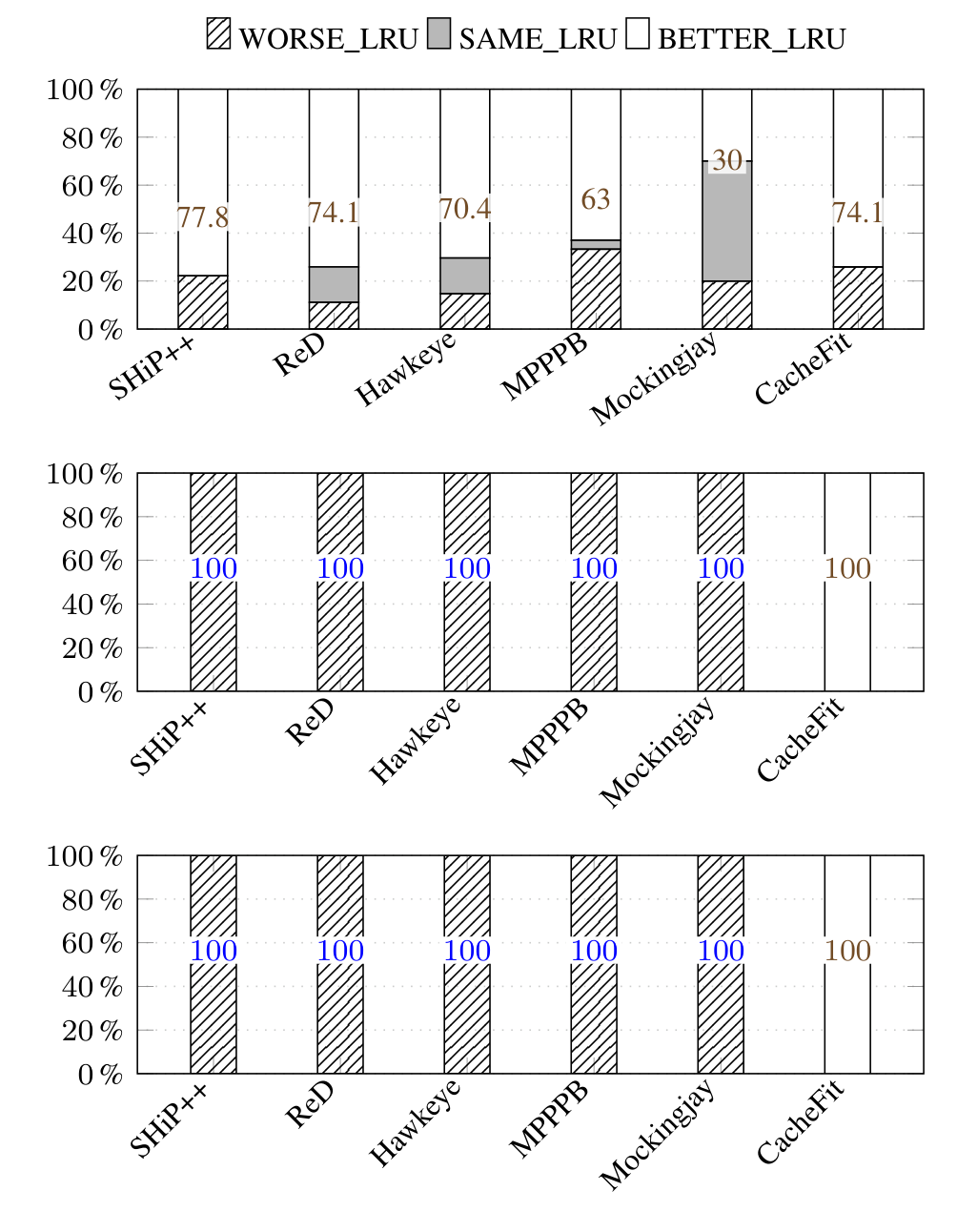
Performance, storage, and power trade-offs

Performance, storage, and power trade-offs. The plots show how frequently each policy performs worse than, similarly to, or better than LRU under three metrics.

The plots show how frequently each policy performs worse than, similarly to, or better than LRU under three metrics.

Figure 8

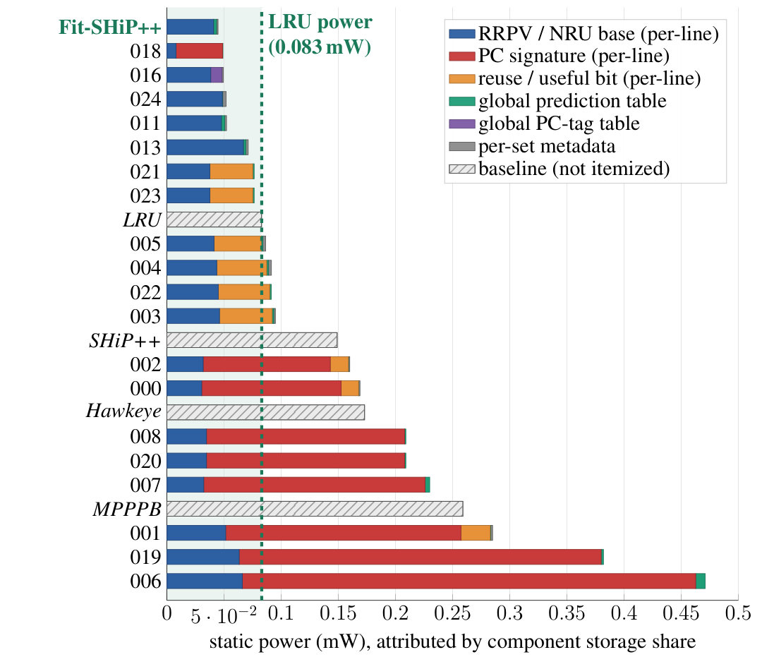
Which components dominate static power?

Which components dominate static power?. HARCOM analytical estimates attribute static power to policy components, including PC-signature arrays.

HARCOM analytical estimates attribute static power to policy components, including PC-signature arrays.

Figure 9

Exploring beyond existing policy designs

Exploring beyond existing policy designs. The plot compares policy families and their positions in the reported design-space analysis.

The plot compares policy families and their positions in the reported design-space analysis.

CACHEFORGE

Generate new cache replacement logic, then learn from its performance.

CACHEFORGE places an LLM inside an iterative generation and evaluation loop to develop C++ cache replacement policies. CRC-2 ChampSim evaluates each candidate, while structural checks and hardware-aware objectives guide the search toward compact, practical designs.

Key findingGenerate · evaluate · refine

A simulator-guided loop explores CPU cache replacement mechanisms.

Paper · PDFarXiv recordBibTeX

Significant findings

10.15%

Higher IPC than LRU

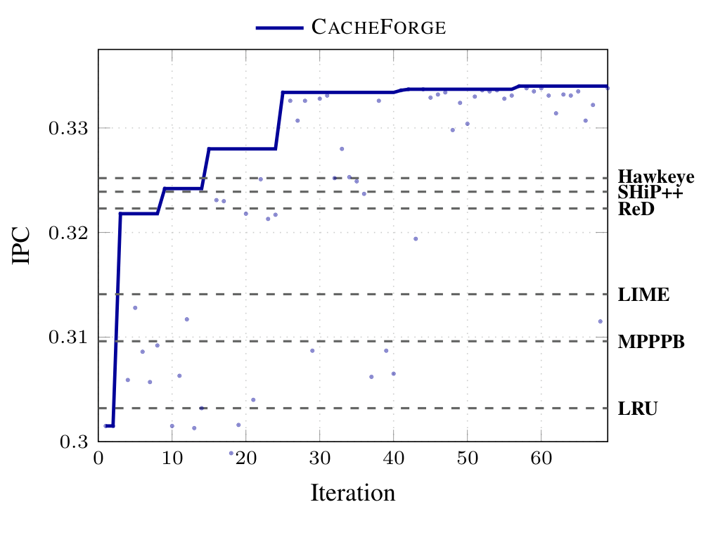
On the evaluated memory-intensive workloads, CACHEFORGE improves instructions per cycle by 10.15% over LRU and 7.89% over MPPPB.

27.36%

Higher total hit rate than MPPPB

Across SPEC CPU2006, the paper reports a 27.36% relative total hit-rate improvement over MPPPB, and 5.73% over LRU.

New decision logic

Search beyond fixed policy structures

The loop generates C++ replacement mechanisms and evaluates each candidate, rather than only tuning parameters in a fixed design.

Hardware budgets

Compact policies guided by constraints

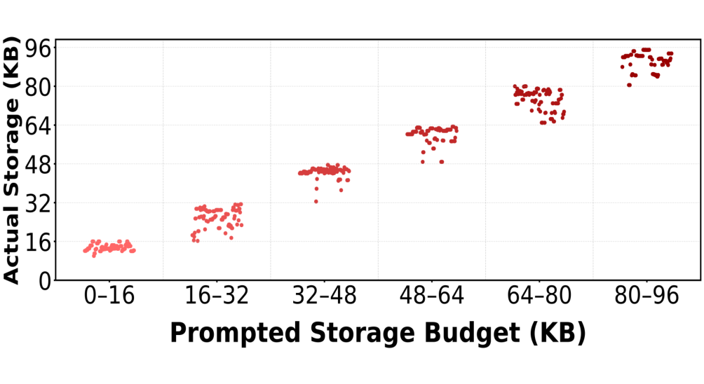
Storage-budget experiments show how the requested overhead budget guides the generated policy’s storage requirements.

Explore the evidence

8 figures · Select a preview to enlarge
Figure 1

The CACHEFORGE design loop

The CACHEFORGE design loop. An LLM proposes replacement logic, simulation evaluates it, and feedback guides the next iteration.

An LLM proposes replacement logic, simulation evaluates it, and feedback guides the next iteration.

Figure 3

IPC optimization over iterations

IPC optimization over iterations. The reported search improves IPC as successive policies are generated and evaluated.

The reported search improves IPC as successive policies are generated and evaluated.

Figure 4

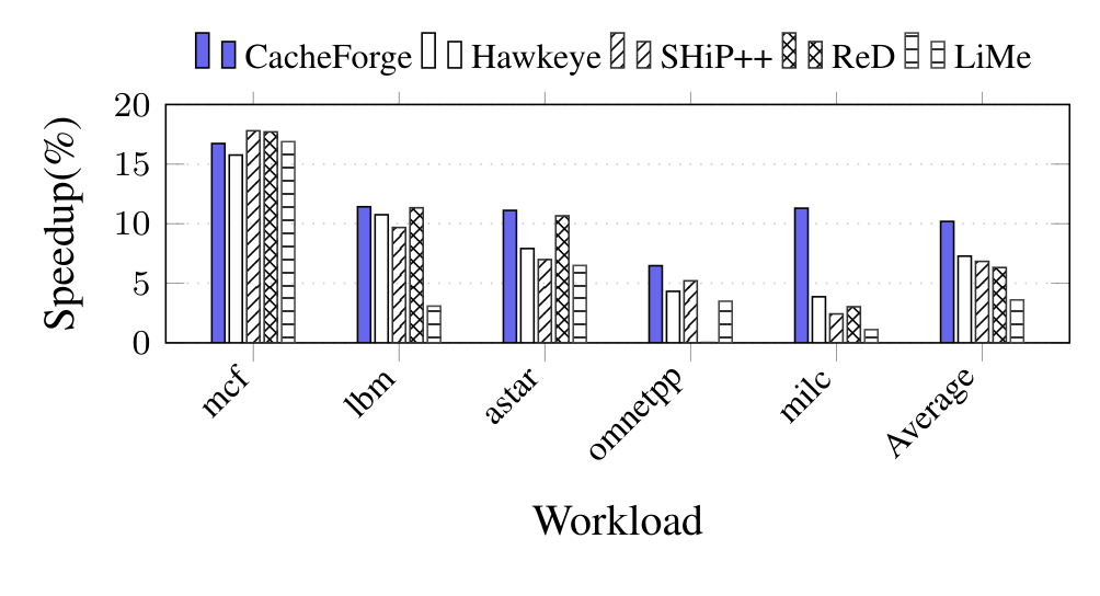
Performance across SPEC workloads

Performance across SPEC workloads. CACHEFORGE policies are compared with LRU and other replacement-policy baselines across the evaluated workloads.

CACHEFORGE policies are compared with LRU and other replacement-policy baselines across the evaluated workloads.

Figure 5

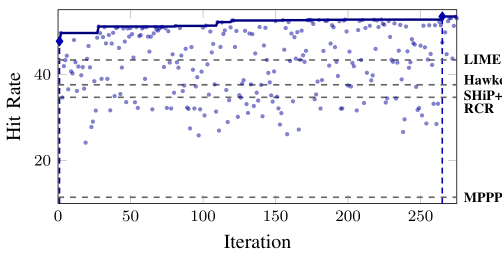
Cache hit rate during the search

Cache hit rate during the search. The trace shows hit-rate progress and the transition between the LLMs used in the reported search.

The trace shows hit-rate progress and the transition between the LLMs used in the reported search.

Figure 6

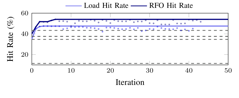
Load and RFO hit-rate evolution

Load and RFO hit-rate evolution. The plot separates load and read-for-ownership behavior as replacement policies evolve.

The plot separates load and read-for-ownership behavior as replacement policies evolve.

Figure 8

Alignment with storage budgets

Alignment with storage budgets. Generated policies are evaluated against the requested storage-overhead budgets.

Generated policies are evaluated against the requested storage-overhead budgets.

Figure 9

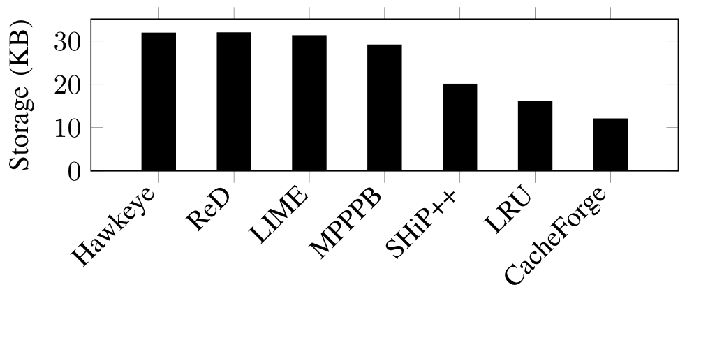
Storage overhead of generated policies

Storage overhead of generated policies. Storage requirements of proposed policies are compared with established baselines.

Storage requirements of proposed policies are compared with established baselines.

Figure 11

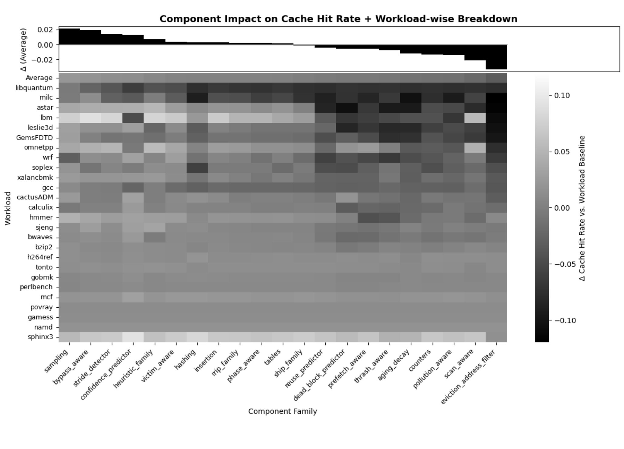
Which policy components improve hit rate?

Which policy components improve hit rate?. The heatmap compares explored components and their effects across evaluated workloads.

The heatmap compares explored components and their effects across evaluated workloads.

CacheMind

Move from counting cache misses to explaining why they happen.

CacheMind lets architects ask natural-language questions about cache behavior and receive answers tied to simulation traces. Task-specific retrieval selects the events needed to explain an eviction, compare policies, or investigate a program counter. CacheMindBench tests both trace-grounded analysis and policy reasoning.

Key finding89.33%

Ranger’s score on 75 unseen trace-grounded questions; 64.80% on the 25 policy-reasoning questions.

Paper · PDFSlidesCodeBibTeX
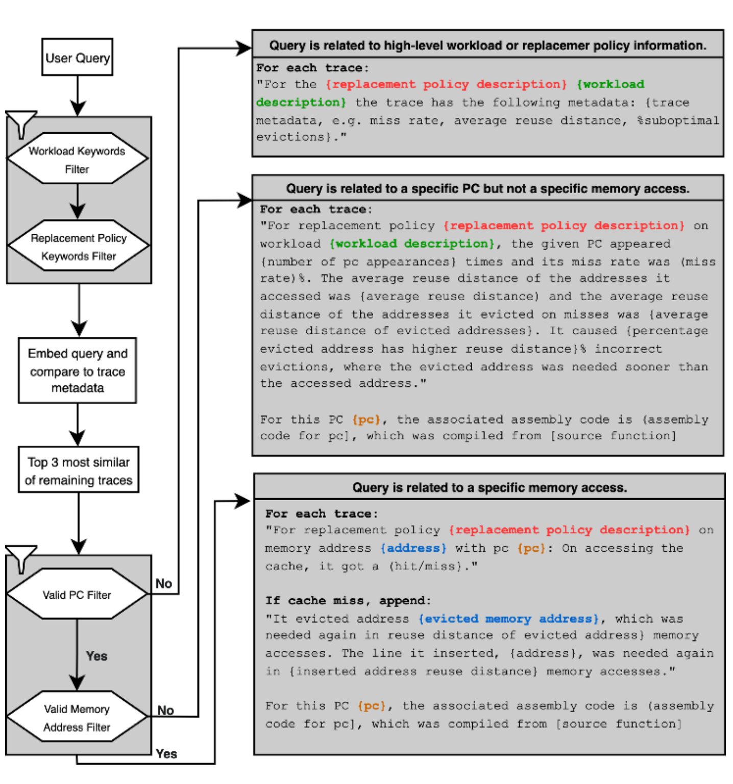
CacheMind retrieval workflow filters a user query by workload and replacement policy, then retrieves trace evidence at the program-counter or memory-address level.

The retrieval pipeline narrows raw traces to the workload, policy, program counter, and memory access relevant to a question.

Figure 1 · ASPLOS 2026Full-size figureSource page

Explore the evidence

1 figures · Select a preview to enlarge
Figure 4

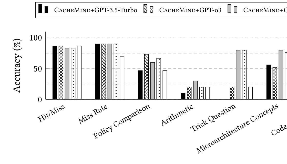
Accuracy across CacheMindBench categories

A grouped bar chart compares CacheMind accuracy across benchmark categories, including hit or miss, miss rate, policy comparison, arithmetic, and ticket questions.

The chart compares CacheMind configurations and language-model backends across trace-grounded and policy-reasoning tasks.

Composite Instruction Prefetching

Combine complementary predictors to keep the front end supplied.

Different instruction prefetchers recognize different program patterns. Composite prefetching combines their strengths through a shared selection mechanism. The framework searches for effective combinations under a fixed metadata budget, with especially useful gains when storage is constrained.

Key findingComplementary coverage

The evaluated composites outperform individual prefetchers across the tested storage budgets.

Paper · PDFBibTeX
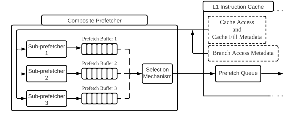
Composite prefetcher architecture connects three sub-prefetchers and buffers to a shared selection mechanism and instruction-cache prefetch queue.

Multiple sub-prefetchers keep separate buffers, while a selection mechanism chooses which requests enter the instruction-cache prefetch queue.

Figure 2 · ICCD 2022Full-size figureSource page

Explore the evidence

1 figures · Select a preview to enlarge
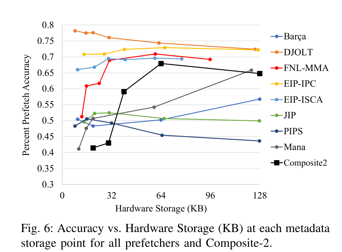
Figure 6

Prefetch accuracy under different storage budgets

A line chart compares instruction prefetch accuracy across hardware-storage budgets for individual prefetchers and Composite-2.

Each curve reports a prefetcher’s accuracy as the available metadata storage changes; the composite is compared with its components.

Dynamic Set Stealing

Let competing cache policies earn the space they use.

A fixed allocation of cache sets can waste capacity when one replacement policy better fits the current workload. Set Stealing with Perceptron Tables reallocates sets among competing policies while learning reuse behavior, adapting both the prediction and the resources behind it.

Key finding9.45%

Geometric-mean speedup over LRU across 81 SPEC workloads with a 2 MB last-level cache.

Paper · PDFBibTeX
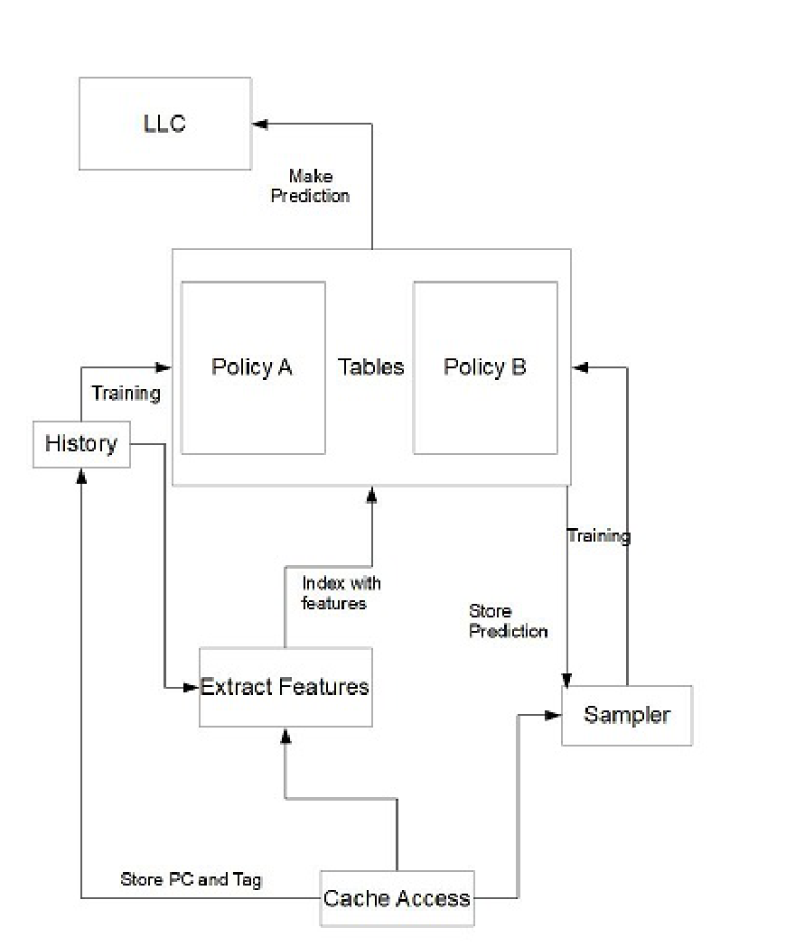
Set-stealing datapath: cache-access features index competing policy tables, store predictions, and train policies through a sampler.

The datapath connects feature extraction, policy predictions, and training so multiple policies can compete within one cache.

Figure 2 · SBAC-PAD 2022Full-size figureSource page

Explore the evidence

1 figures · Select a preview to enlarge
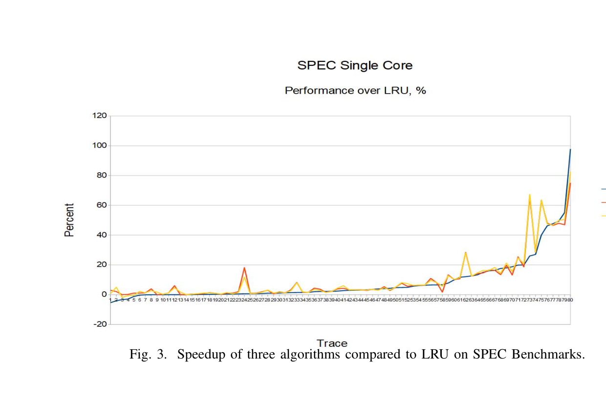
Figure 3

Speedup across SPEC workloads

A line chart shows speedup over LRU for three set-stealing algorithms across SPEC CPU benchmarks.

The plot compares three set-stealing algorithms with LRU across the evaluated SPEC CPU traces.

CHiRP

Keep address translations that are likely to be used again.

Translation lookaside buffers have limited space, and a miss can trigger an expensive page-table walk. CHiRP uses control-flow history to predict which translations will be reused. Its replacement policy is tailored to TLB behavior instead of directly reusing a data-cache policy.

Key finding28.21% fewer misses

Average reduction in misses per 1,000 instructions versus LRU for the evaluated 1,024-entry, 8-way L2 TLB.

Paper · PDFBibTeX
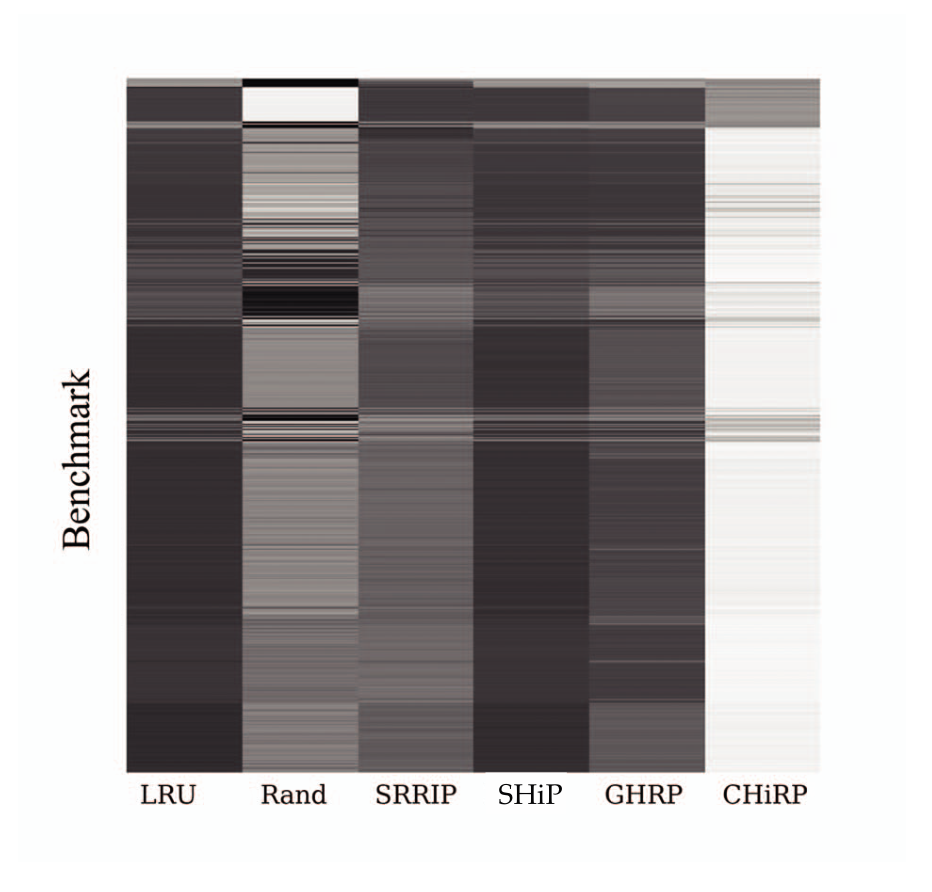
Heatmap of TLB efficiency across 870 benchmarks: CHiRP has lighter regions than LRU, random replacement, SRRIP, SHiP and GHRP.

Lighter regions indicate more useful live entries. CHiRP keeps more reusable translations across the 870 evaluated benchmarks.

Figure 1 · MICRO 2020Full-size figureSource page

Explore the evidence

1 figures · Select a preview to enlarge
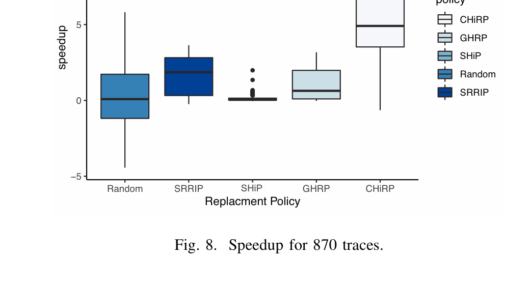
Figure 8

Speedup across 870 traces

A box plot compares speedup across 870 traces for CHiRP, GHRP, SHiP, random replacement, and SRRIP.

The box plot summarizes speedup for the evaluated TLB replacement policies across 870 traces.

Bit-Level Perceptron Prediction

Learn a branch destination one bit at a time.

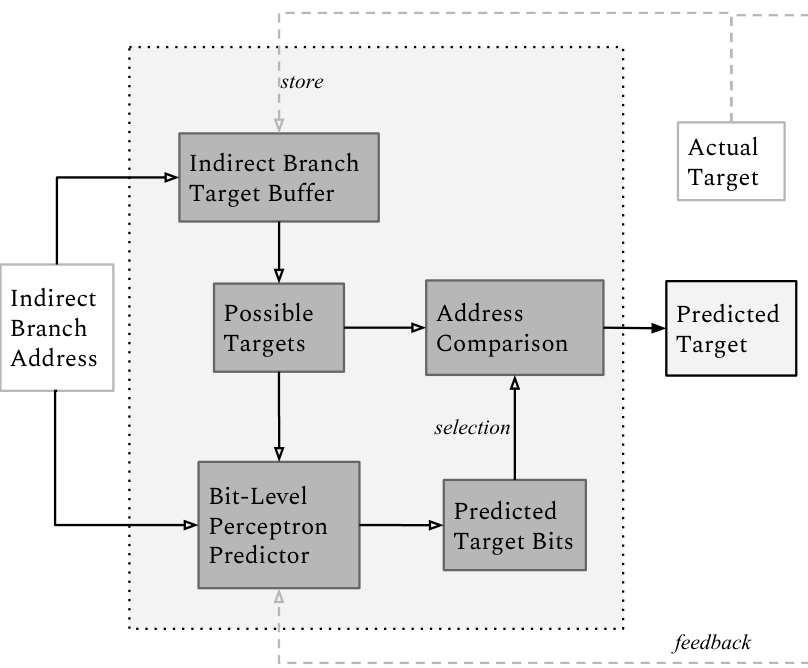
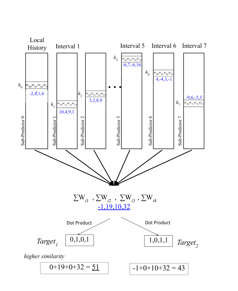
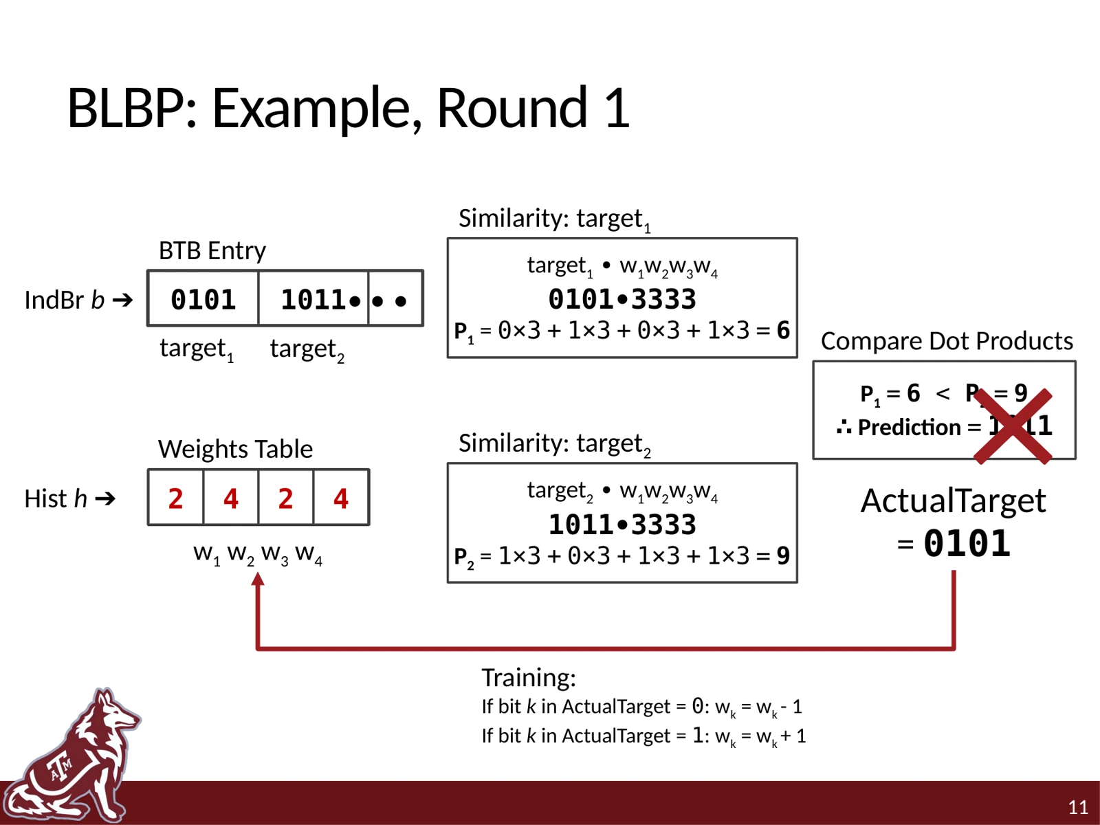
Indirect branches—such as calls through function pointers—can lead to several destinations, and their next target is hard to infer from the branch address alone. BLBP learns individual target-address bits from recent branch history using eight perceptron-based subpredictors, each looking at a different history view. It adds their scores into a bit pattern, compares that pattern with destinations already observed for the branch, and predicts the closest match. After the branch resolves, the actual target trains the weights so future predictions improve. This means BLBP predicts among known targets rather than trying to invent an arbitrary address.

Key findingAbout 5% fewer mispredictions

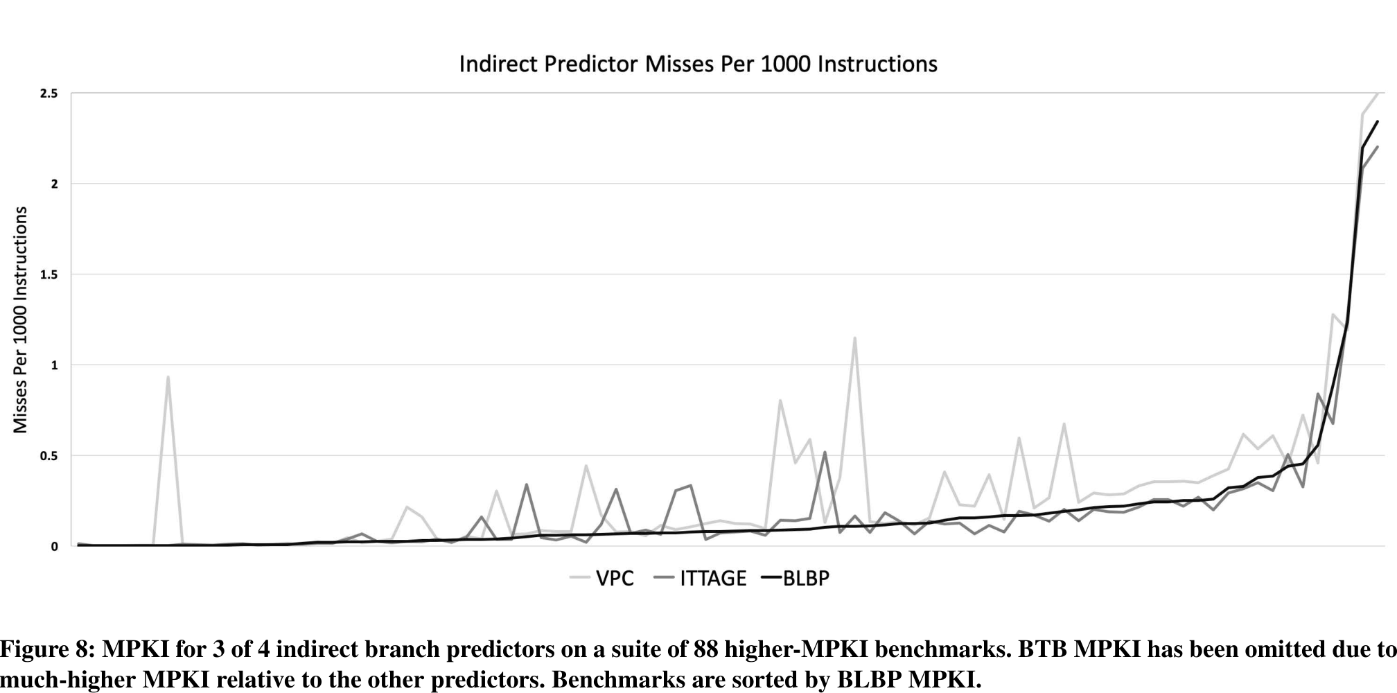
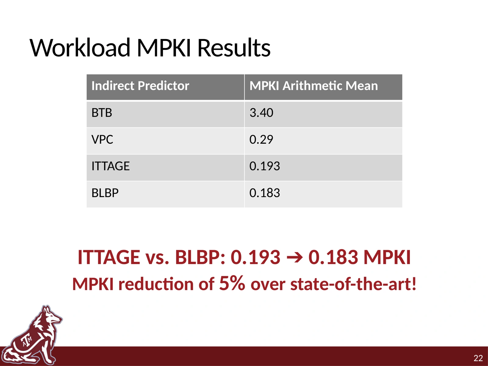
Across 88 higher-MPKI workloads, average indirect-branch MPKI fell from 0.193 with ITTAGE to 0.183 with BLBP (about 5% fewer misses) at a similar hardware budget.

Paper · PDFSlidesBibTeX
BLBP overview: branch history feeds bit-level perceptrons; their predicted target bits are matched against the branch's stored target addresses.

The paper’s overview shows how BLBP scores target-address bits, compares the prediction against candidate destinations, and selects the closest match.

Figure 2 · ISCA 2019Full-size figureSource page

Explore the evidence

5 figures · Select a preview to enlarge
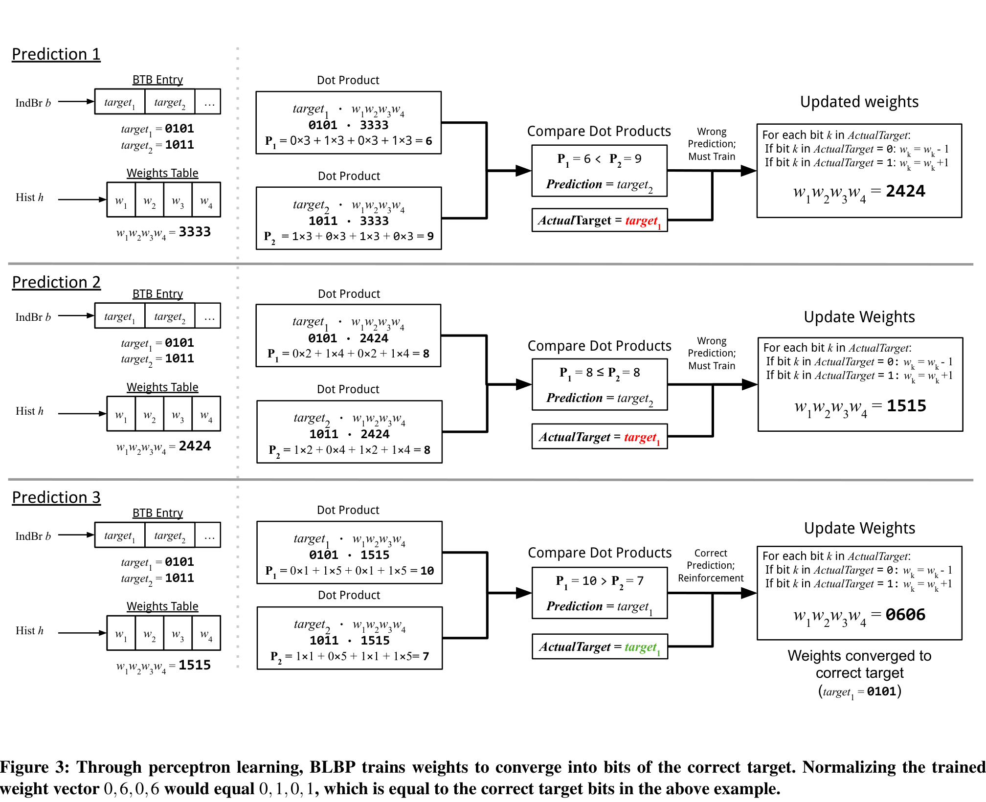
Figure 3

Learning target bits through perceptron updates

Three stages of BLBP training show target-bit predictions, dot-product comparisons, and weight updates converging to the actual target.

Across successive predictions, the weight vector is adjusted using the actual destination. The normalized weights converge toward the target’s bit pattern.

Figure 4

Combining several history views

BLBP prediction diagram shows eight history subpredictors feeding summed bit scores, which are compared with two candidate targets.

Eight history-based subpredictors contribute scores for each target bit. BLBP aggregates those scores, compares each observed target, and chooses the target with the strongest match.

Figure 7

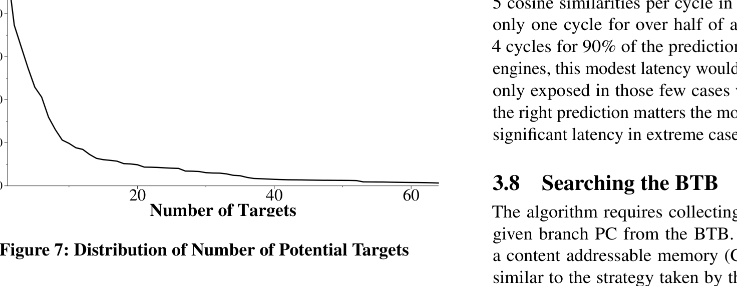
How many possible targets do branches have?

A descending distribution curve shows the share of indirect branches by number of observed possible targets, with most branches having few targets.

Most evaluated indirect branches have relatively few observed destinations; only a small fraction have many. This makes comparing the predicted bit pattern with the branch’s observed targets practical.

Figure 8

Prediction misses across 88 workloads

Line chart compares indirect-branch MPKI for BLBP, ITTAGE, and VPC across 88 workloads sorted by BLBP performance.

The paper compares misses per 1,000 instructions (MPKI) for BLBP, ITTAGE, and VPC across 88 workloads. BLBP achieves 0.183 average MPKI versus 0.193 for ITTAGE in the study, about a 5% reduction at a similar hardware budget.

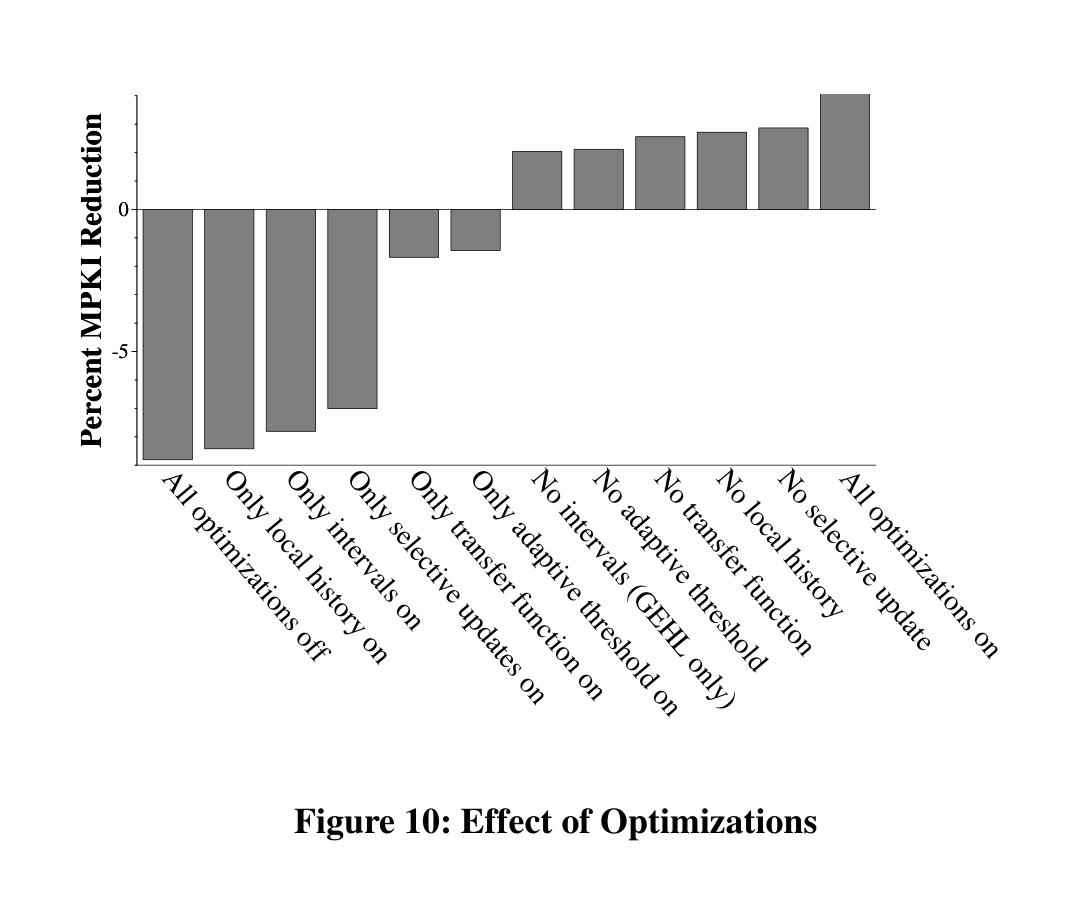
Figure 10

How each predictor optimization affects MPKI

A bar chart shows the percent change in indirect branch prediction MPKI when BLBP optimizations are individually disabled or enabled.

The ablation compares prediction error as individual BLBP optimizations are enabled or disabled.

From the ISCA 2019 talk

The idea, step by step

Three selected slides show the bit-level predictor, one training example, and the measured comparison.

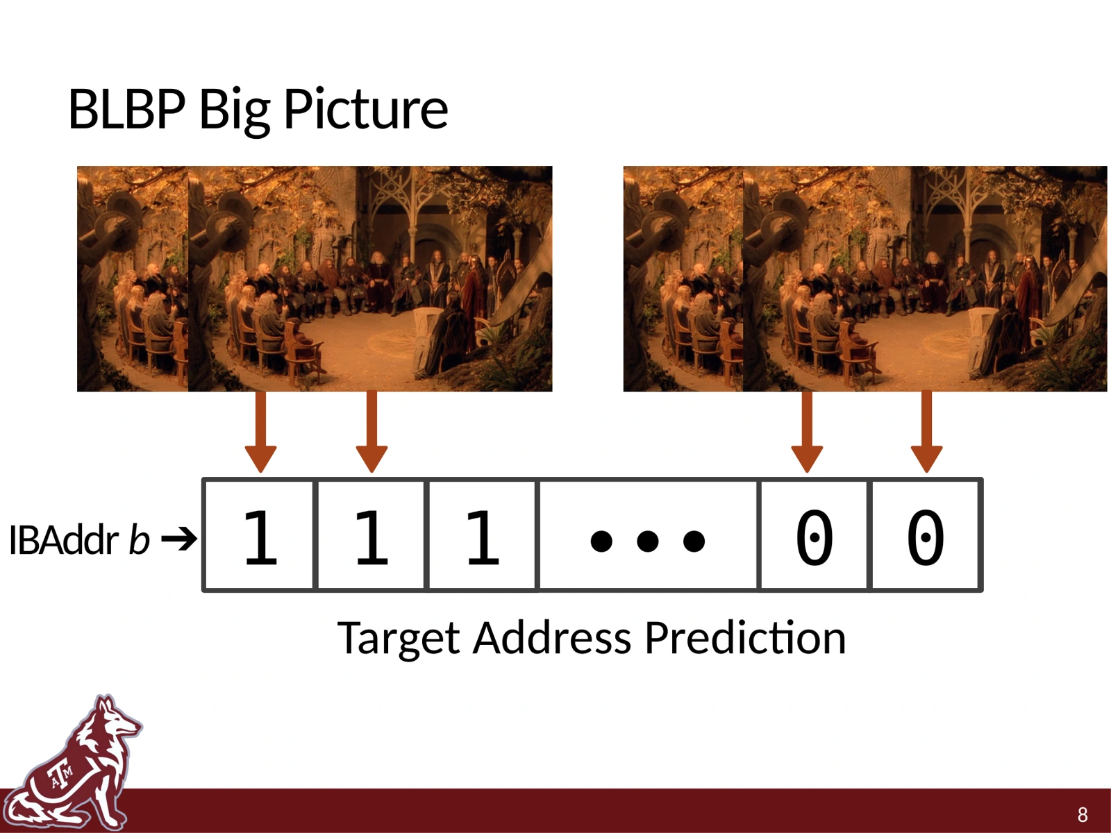
Talk slide 8

BLBP at a glance

ISCA 2019 presentation slide 8: BLBP predicts an indirect branch target as a sequence of address bits.

The talk’s overview introduces BLBP as bit-level target-address prediction for indirect branches.

Talk slide 11

A worked prediction and update

ISCA 2019 presentation slide 11: numerical example of BLBP candidate-target dot products, a wrong prediction, and weight training.

This slide walks through candidate-target scores, shows a prediction, then updates weights using the actual target.

Talk slide 22

The evaluated result

ISCA 2019 presentation slide 22: table of indirect predictor average MPKI, showing BLBP at 0.183 and ITTAGE at 0.193.

The presentation reports average MPKI of 0.183 for BLBP and 0.193 for ITTAGE, a 5% reduction in this evaluation.

Global History Reuse Prediction

Replace entries by expected reuse, not just by recency.

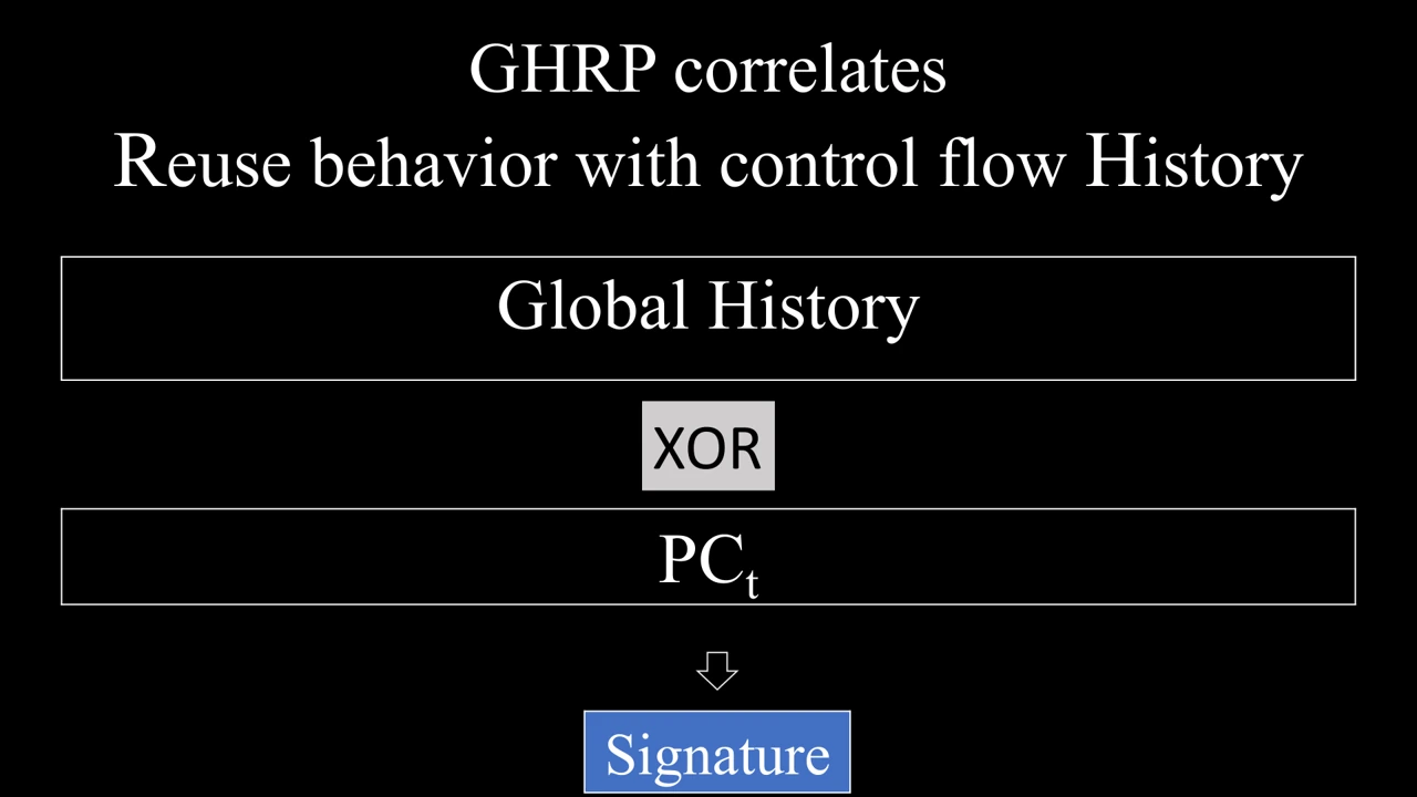
GHRP uses the history of instruction addresses to predict which instruction-cache blocks and branch-target-buffer entries will no longer be useful. Replacing or bypassing those entries makes limited front-end storage available to instructions that are likely to return.

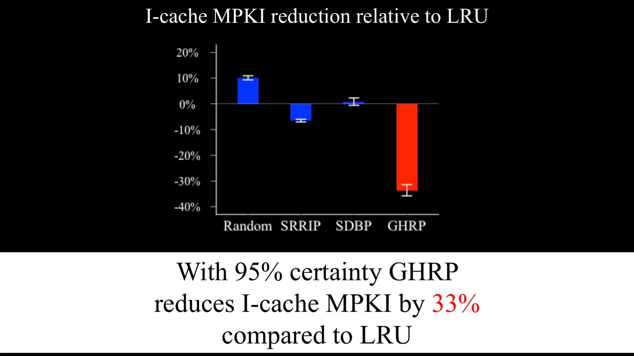
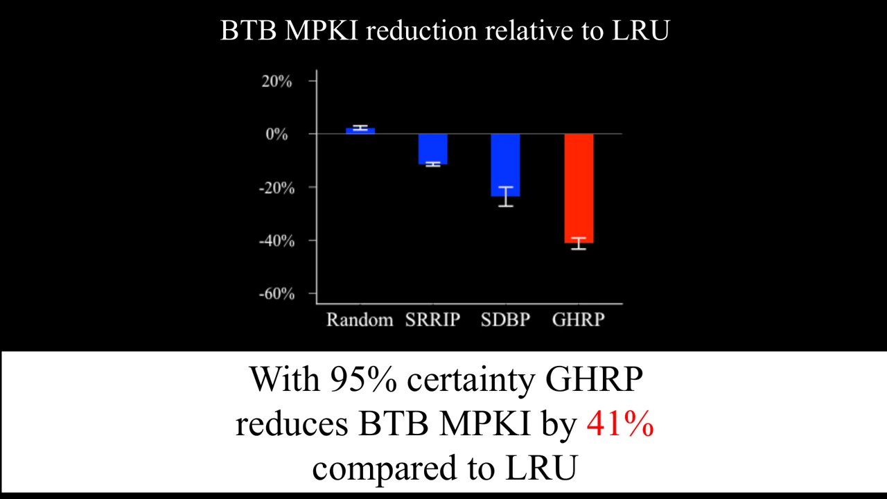
Key finding18% / 30%

Average miss reductions versus LRU for the evaluated 64 KB instruction cache and 4K-entry branch target buffer, respectively.

Paper · PDFSlidesLightning talk · PowerPointBibTeX
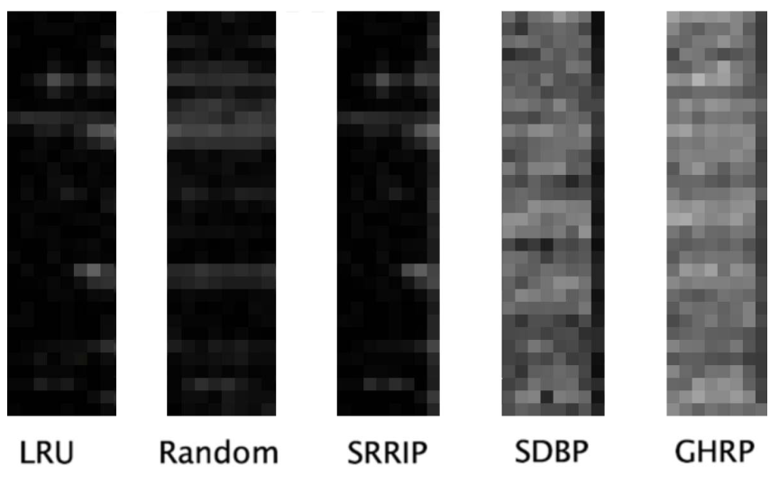
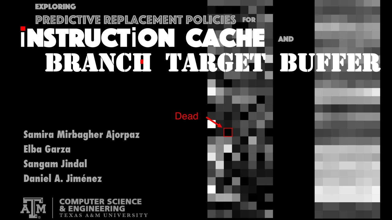
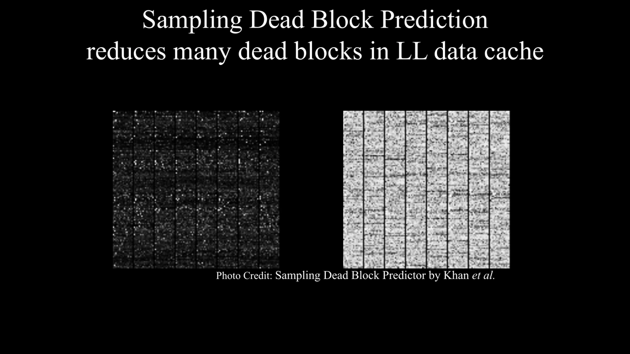
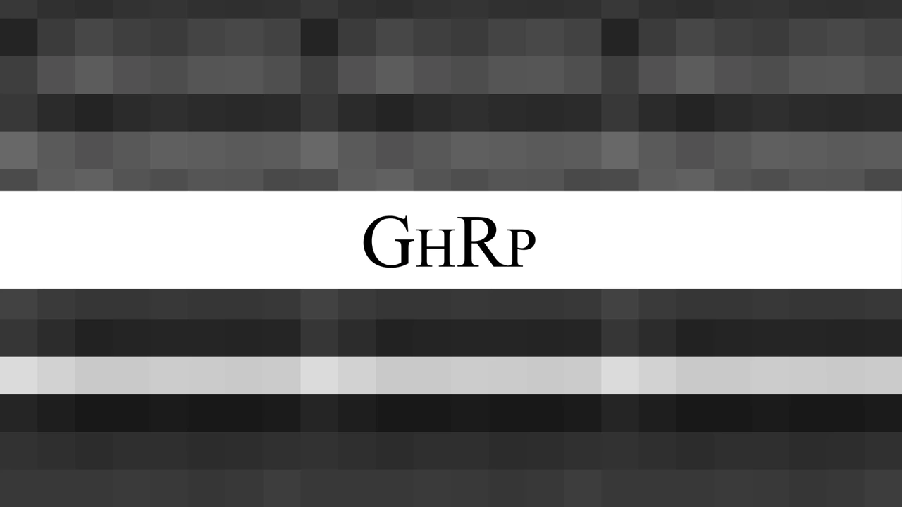
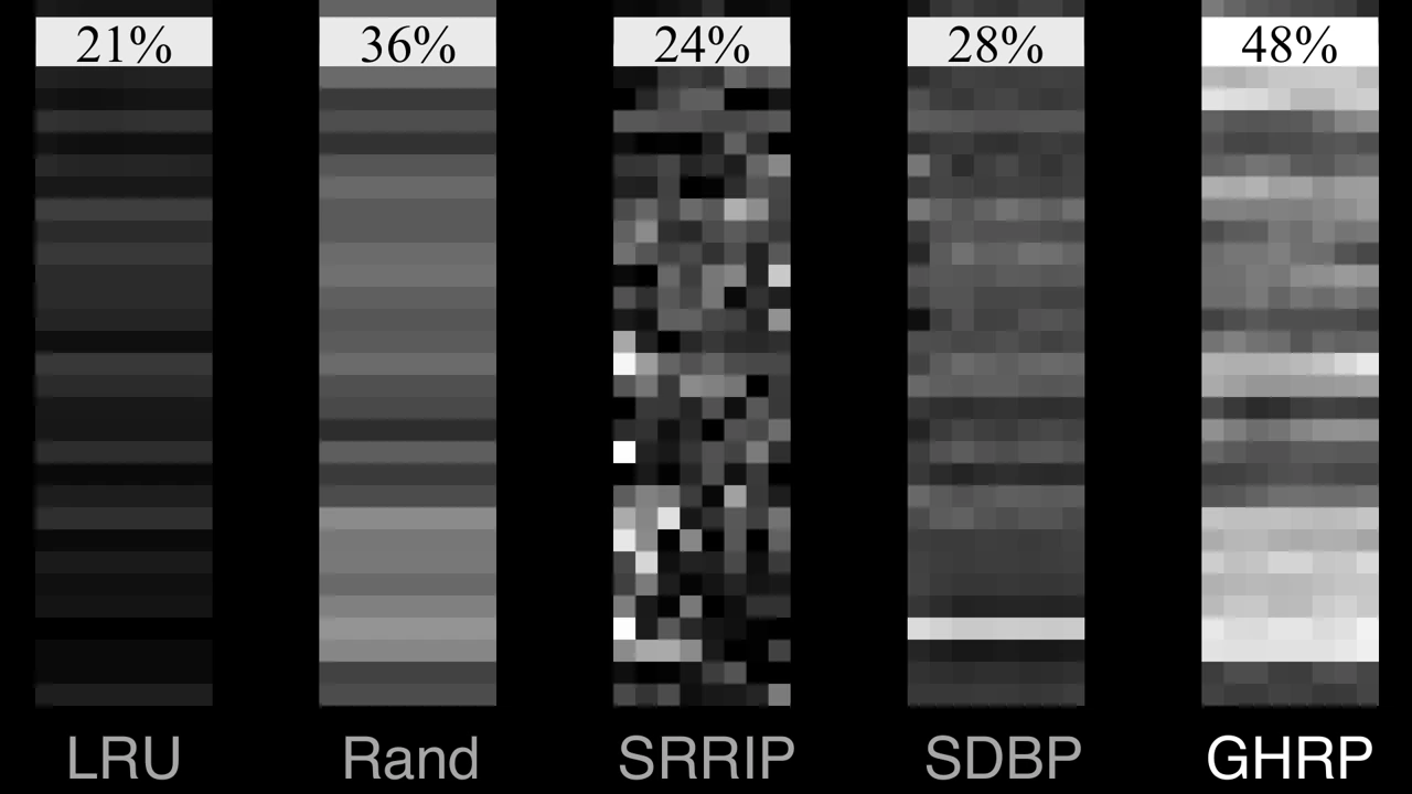
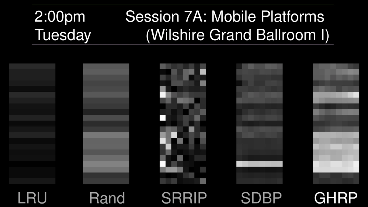
Five heatmaps compare branch-target-buffer efficiency; GHRP is lighter than LRU, random replacement, SRRIP and SDBP for the illustrated trace.

In this branch-target-buffer trace, lighter pixels mean entries spend more time live. GHRP retains useful information for longer.

Figure 5 · ISCA 2018Full-size figureSource page

Explore the evidence

1 figures · Select a preview to enlarge
Figure 3

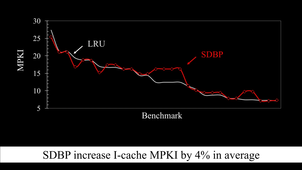
Instruction-cache miss rates across policies

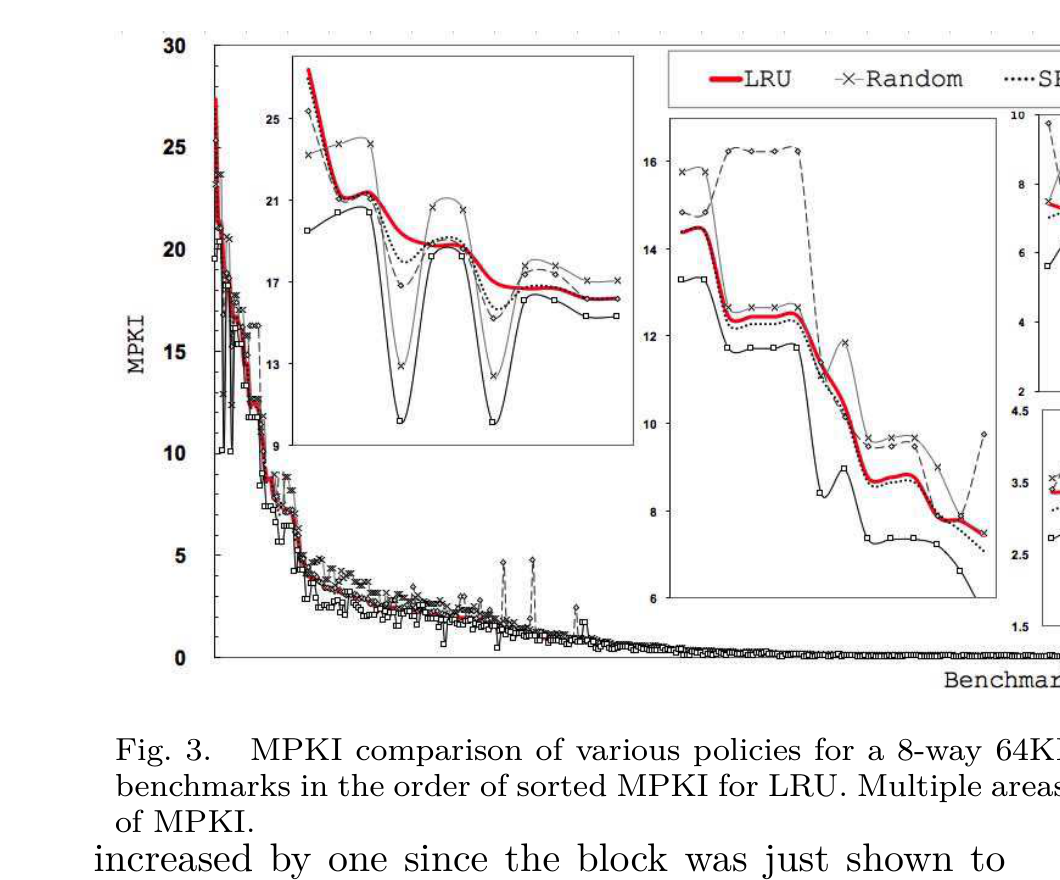
A multi-panel line chart compares instruction-cache MPKI across benchmarks for LRU, random, SRRIP, SDBP, and predictive policies.

The comparison plots instruction-cache MPKI for the evaluated replacement policies over the benchmark suite.

Full presentation
28 slides
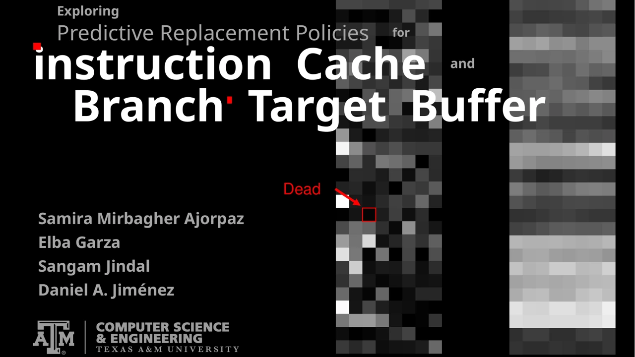
ISCA 2018 full presentation slide 1: Opening. The problem: dead cache blocks
01
Opening

The problem: dead cache blocks

Open slide at full size ↗
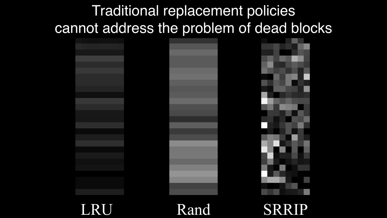
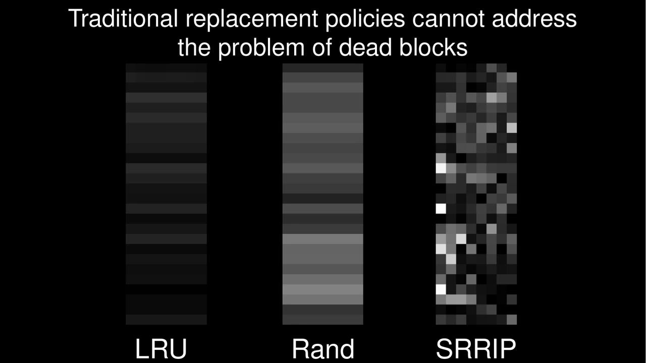
ISCA 2018 full presentation slide 2: Traditional replacement policies. LRU, random replacement, and SRRIP
02
Traditional replacement policies

LRU, random replacement, and SRRIP

Open slide at full size ↗
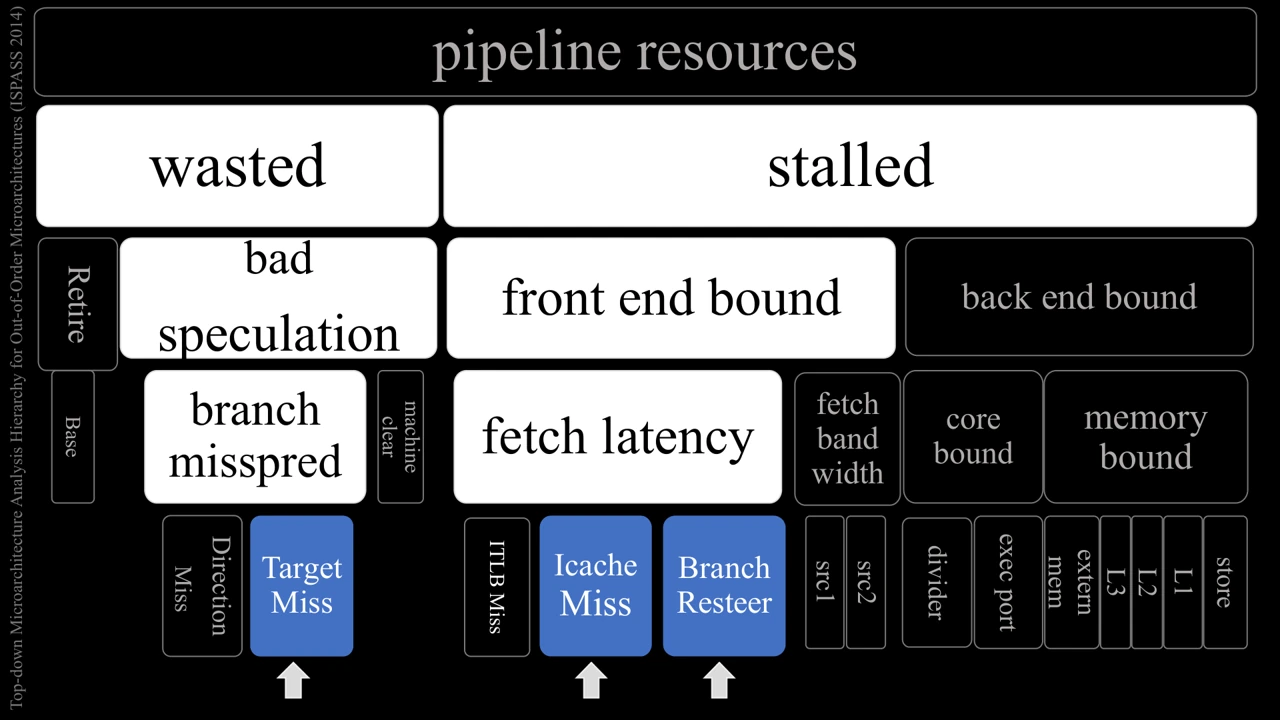
ISCA 2018 full presentation slide 3: Where execution time is lost. Top-down breakdown highlights front-end stalls and misspeculation.
03
Where execution time is lost

Top-down breakdown highlights front-end stalls and misspeculation.

Open slide at full size ↗
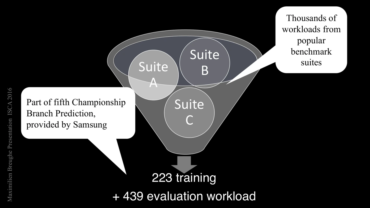
ISCA 2018 full presentation slide 4: Benchmark suites. The evaluation combines training and evaluation workloads.
04
Benchmark suites

The evaluation combines training and evaluation workloads.

Open slide at full size ↗
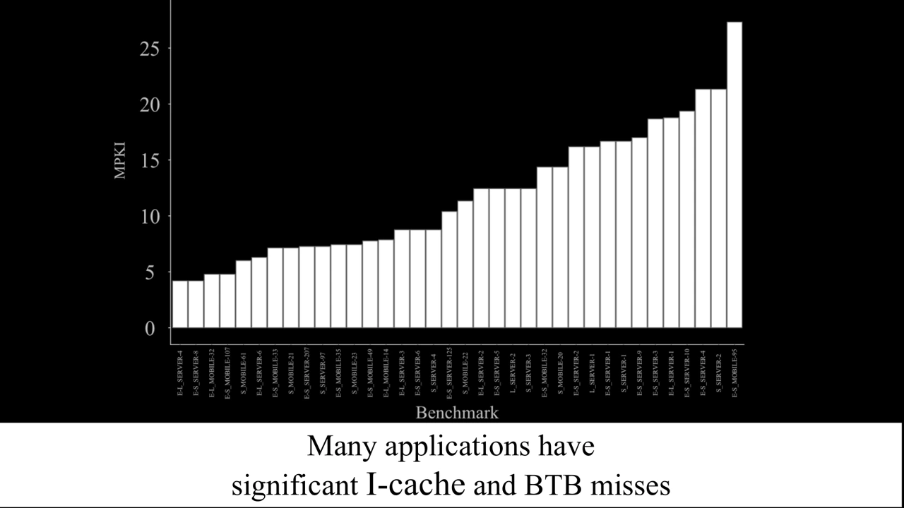
ISCA 2018 full presentation slide 5: Instruction-cache and BTB misses. Many workloads experience meaningful misses in these front-end structures.
05
Instruction-cache and BTB misses

Many workloads experience meaningful misses in these front-end structures.

Open slide at full size ↗
ISCA 2018 full presentation slide 6: Research gap. The talk motivates prediction policies tailored to instruction caches and BTBs.
06
Research gap

The talk motivates prediction policies tailored to instruction caches and BTBs.

Open slide at full size ↗
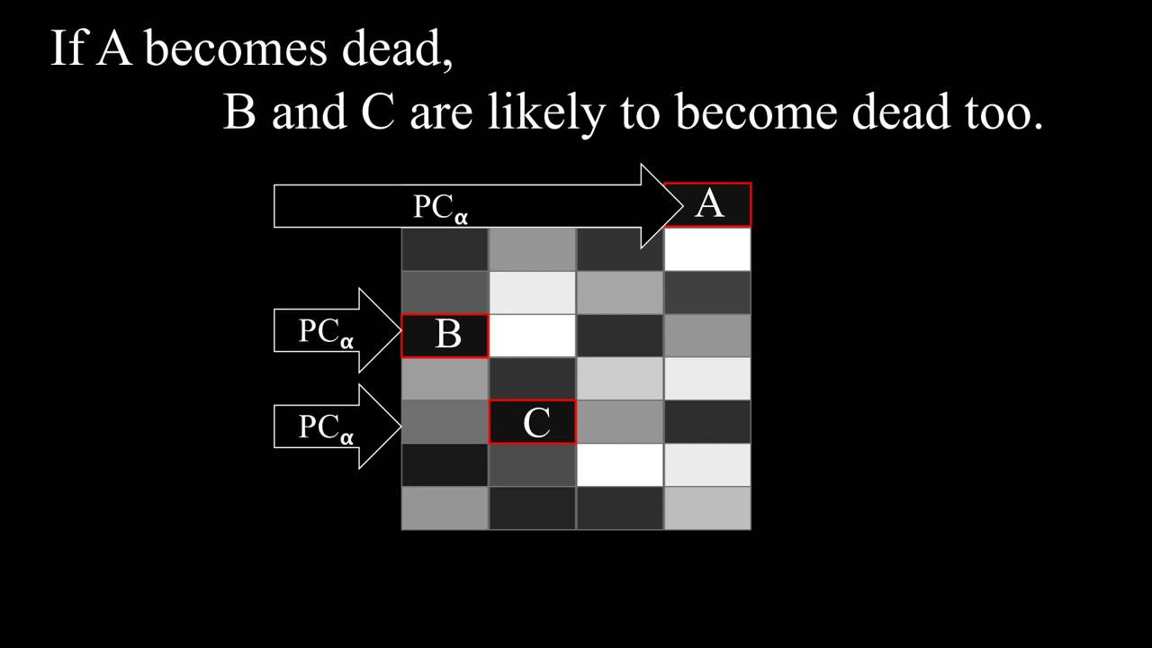
ISCA 2018 full presentation slide 7: Dead-block correlation. The example illustrates how reuse behavior can correlate across nearby instructions.
07
Dead-block correlation

The example illustrates how reuse behavior can correlate across nearby instructions.

Open slide at full size ↗
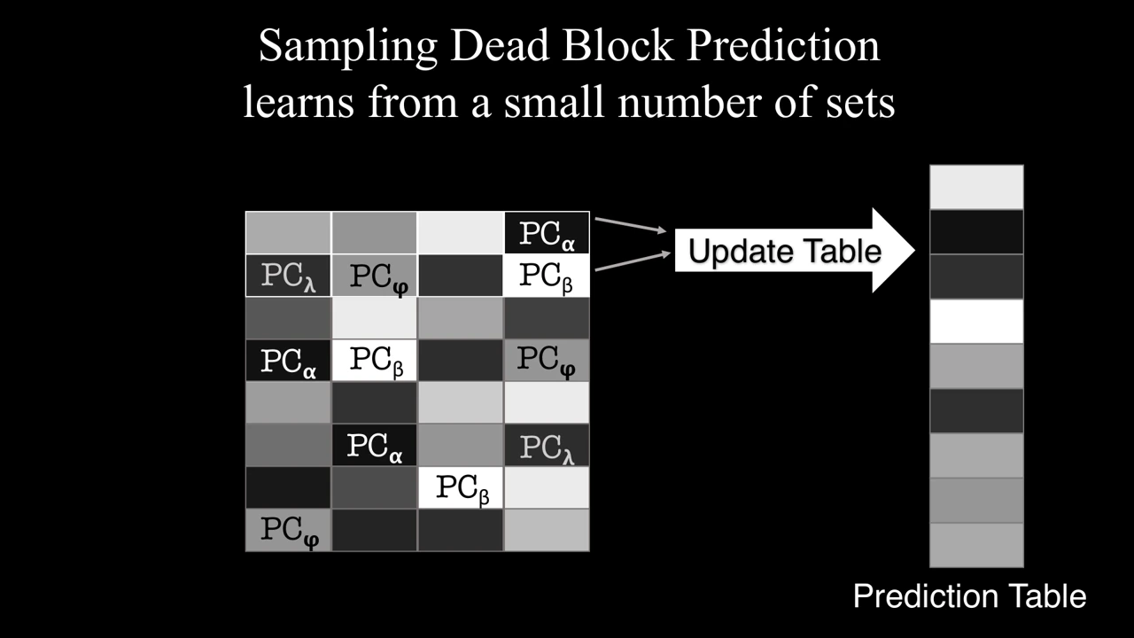
ISCA 2018 full presentation slide 8: Sampling dead-block prediction. A sampler learns block behavior from a small subset of cache sets.
08
Sampling dead-block prediction

A sampler learns block behavior from a small subset of cache sets.

Open slide at full size ↗
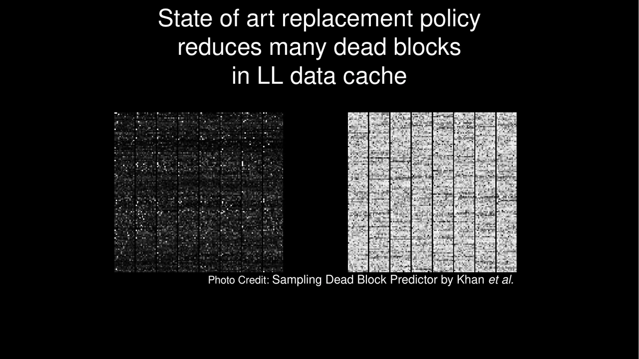
ISCA 2018 full presentation slide 9: SDBP and data caches. Prior dead-block prediction helps data caches, but does not directly solve instruction-cache behavior.
09
SDBP and data caches

Prior dead-block prediction helps data caches, but does not directly solve instruction-cache behavior.

Open slide at full size ↗
ISCA 2018 full presentation slide 10: SDBP on instruction caches. The presented comparison shows why a data-cache policy can perform poorly on instruction caches.
10
SDBP on instruction caches

The presented comparison shows why a data-cache policy can perform poorly on instruction caches.

Open slide at full size ↗
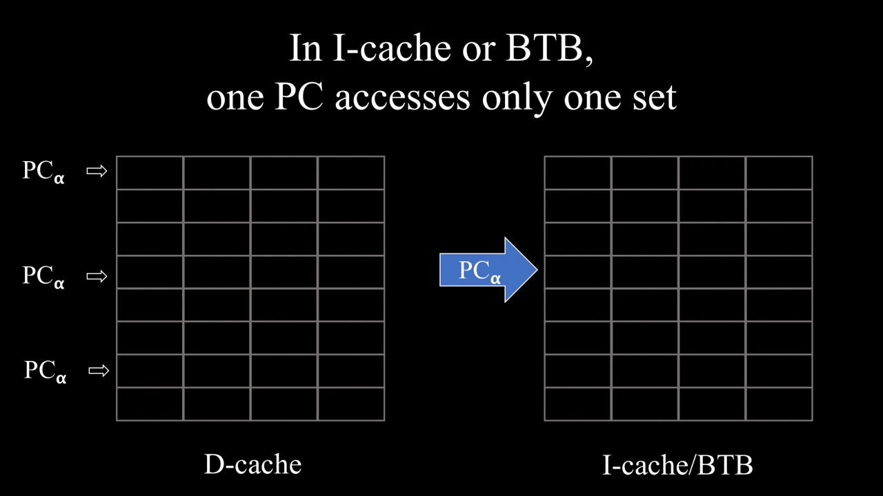
ISCA 2018 full presentation slide 11: One PC, one set. Instruction caches and BTBs have distinct access patterns from data caches.
11
One PC, one set

Instruction caches and BTBs have distinct access patterns from data caches.

Open slide at full size ↗
ISCA 2018 full presentation slide 12: Introducing GHRP. Section divider for Global History Reuse Prediction.
12
Introducing GHRP

Section divider for Global History Reuse Prediction.

Open slide at full size ↗
ISCA 2018 full presentation slide 13: Reuse and control-flow history. GHRP forms a signature by combining the current instruction with recent global branch history.
13
Reuse and control-flow history

GHRP forms a signature by combining the current instruction with recent global branch history.

Open slide at full size ↗
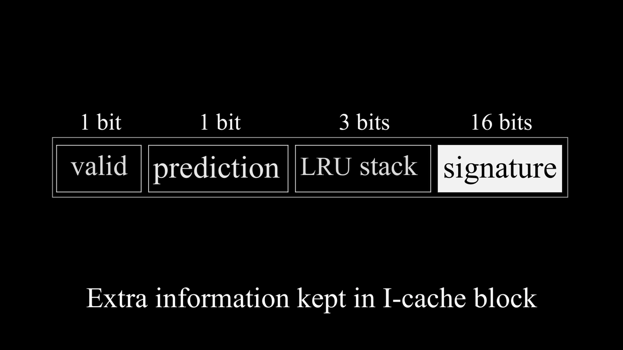
ISCA 2018 full presentation slide 14: Metadata stored with each block. A block keeps a compact reuse signature and prediction metadata.
14
Metadata stored with each block

A block keeps a compact reuse signature and prediction metadata.

Open slide at full size ↗
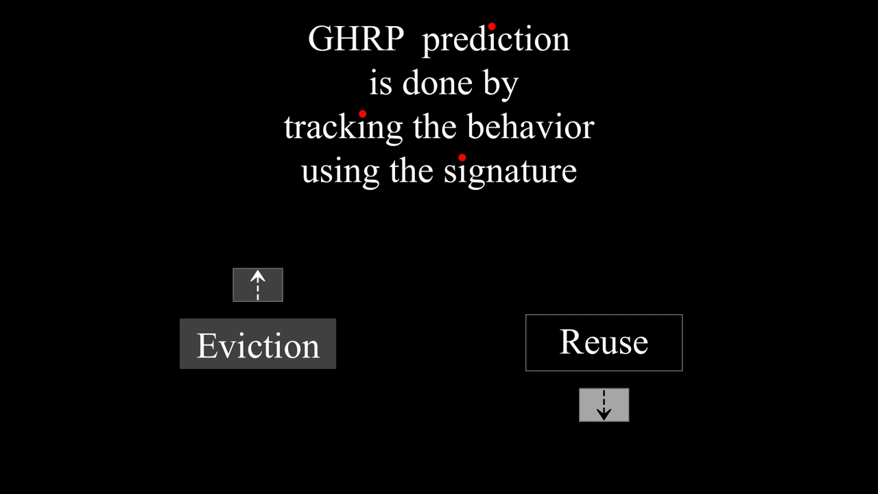
ISCA 2018 full presentation slide 15: Tracking reuse behavior. The signature is used to learn whether a block is likely to be reused or evicted.
15
Tracking reuse behavior

The signature is used to learn whether a block is likely to be reused or evicted.

Open slide at full size ↗
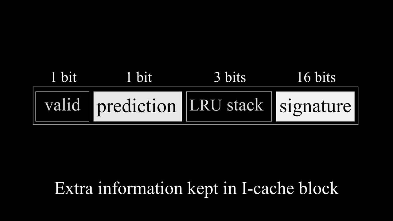
ISCA 2018 full presentation slide 16: Block metadata in context. A second view clarifies where the signature and prediction bits sit in the cache line.
16
Block metadata in context

A second view clarifies where the signature and prediction bits sit in the cache line.

Open slide at full size ↗
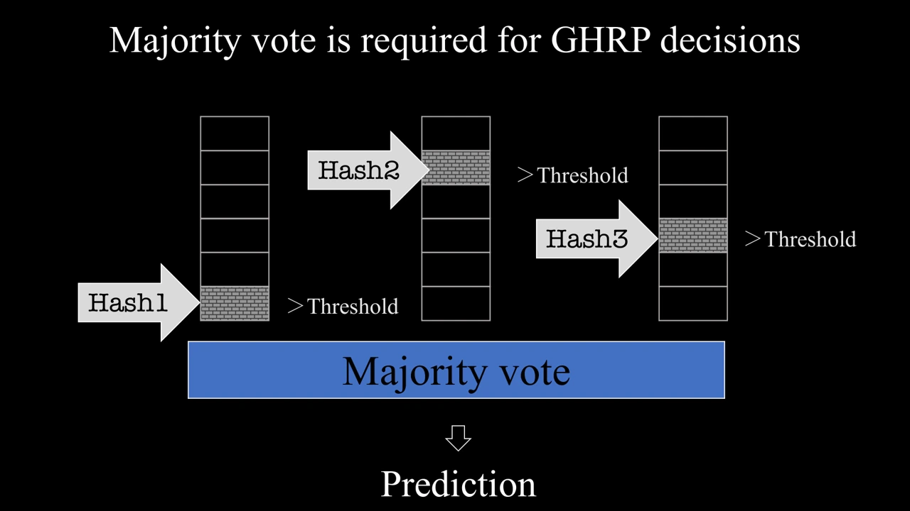
ISCA 2018 full presentation slide 17: Majority-vote prediction. Multiple history-derived predictors vote on the reuse decision.
17
Majority-vote prediction

Multiple history-derived predictors vote on the reuse decision.

Open slide at full size ↗
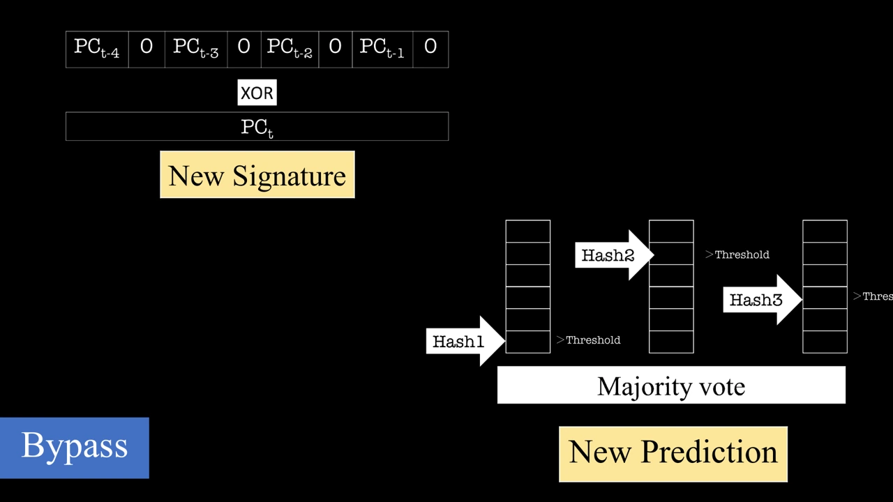
ISCA 2018 full presentation slide 18: Predict and bypass. The predicted reuse outcome determines whether a new block is inserted or bypassed.
18
Predict and bypass

The predicted reuse outcome determines whether a new block is inserted or bypassed.

Open slide at full size ↗
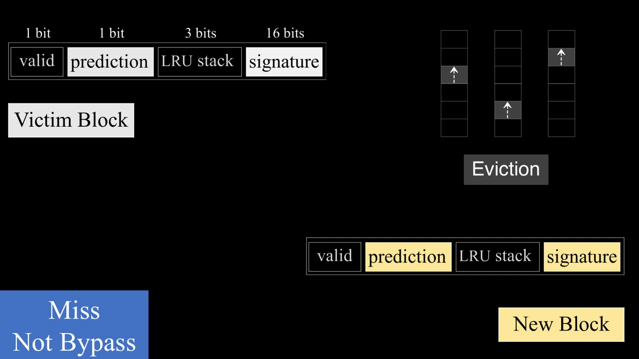
ISCA 2018 full presentation slide 19: Miss and replacement path. The slide walks through allocation after a miss when bypass is not selected.
19
Miss and replacement path

The slide walks through allocation after a miss when bypass is not selected.

Open slide at full size ↗
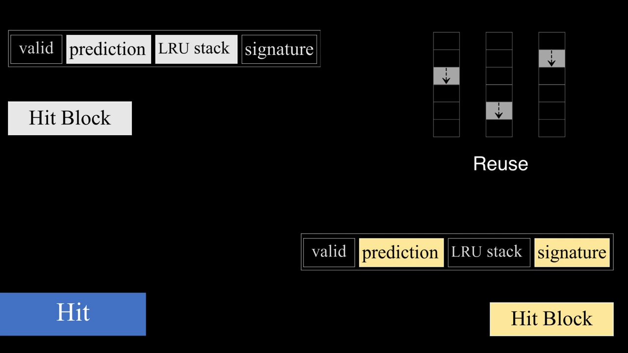
ISCA 2018 full presentation slide 20: Hit and reuse update. A cache hit updates the block’s reuse state.
20
Hit and reuse update

A cache hit updates the block’s reuse state.

Open slide at full size ↗
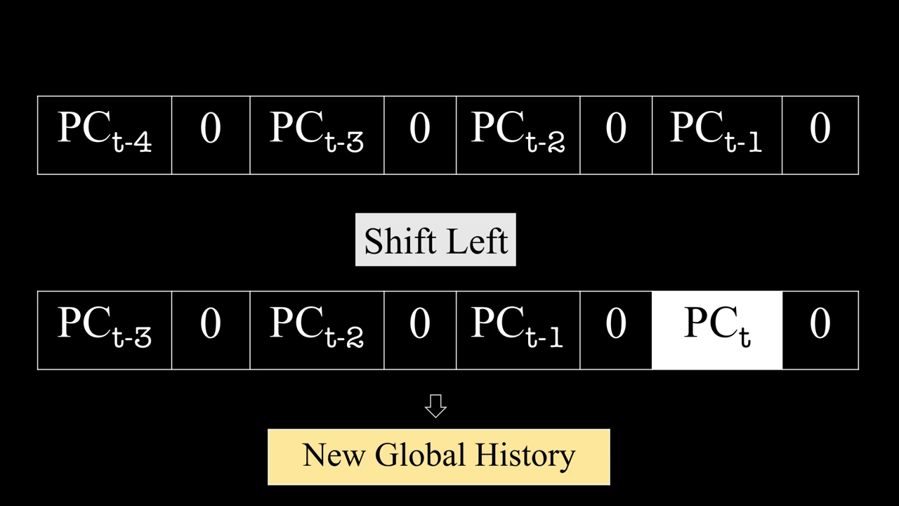
ISCA 2018 full presentation slide 21: Update the global history. The history register shifts in the latest branch information.
21
Update the global history

The history register shifts in the latest branch information.

Open slide at full size ↗
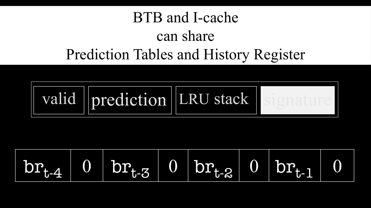
ISCA 2018 full presentation slide 22: Share information across structures. Instruction cache and BTB can share prediction tables and history state.
22
Share information across structures

Instruction cache and BTB can share prediction tables and history state.

Open slide at full size ↗
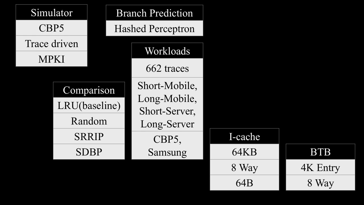
ISCA 2018 full presentation slide 23: Evaluation setup. The talk outlines the simulator, workloads, baselines, and evaluated structures.
23
Evaluation setup

The talk outlines the simulator, workloads, baselines, and evaluated structures.

Open slide at full size ↗
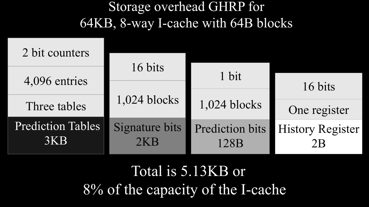
ISCA 2018 full presentation slide 24: Storage overhead. The metadata and prediction tables add about 5.13 KB for the evaluated 64 KB instruction cache.
24
Storage overhead

The metadata and prediction tables add about 5.13 KB for the evaluated 64 KB instruction cache.

Open slide at full size ↗
ISCA 2018 full presentation slide 25: Instruction-cache result. The evaluated results show fewer instruction-cache misses with GHRP than LRU.
25
Instruction-cache result

The evaluated results show fewer instruction-cache misses with GHRP than LRU.

Open slide at full size ↗
ISCA 2018 full presentation slide 26: BTB result. The evaluated results show fewer BTB misses with GHRP than LRU.
26
BTB result

The evaluated results show fewer BTB misses with GHRP than LRU.

Open slide at full size ↗
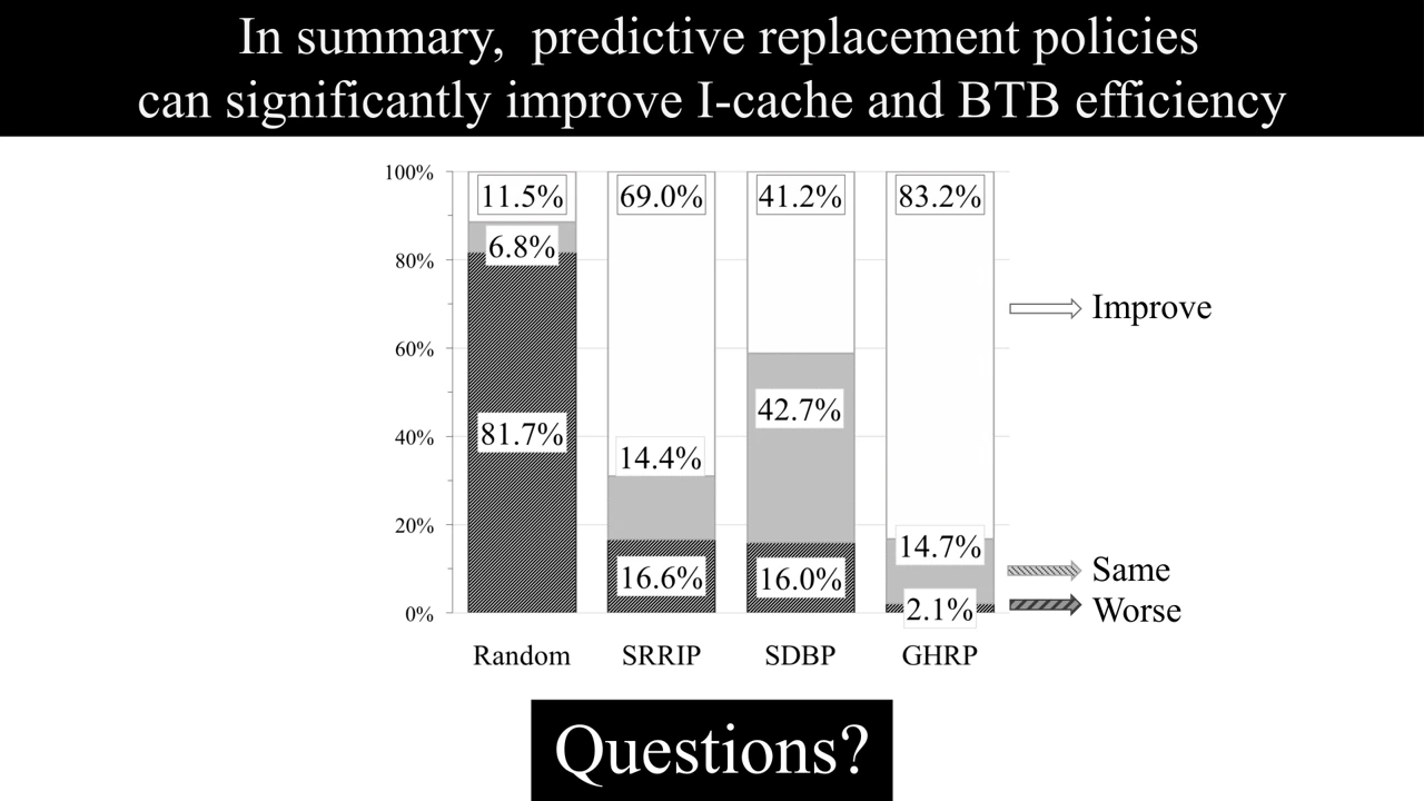
ISCA 2018 full presentation slide 27: Across-policy comparison. GHRP is compared with LRU, random, SRRIP, and SDBP.
27
Across-policy comparison

GHRP is compared with LRU, random, SRRIP, and SDBP.

Open slide at full size ↗
ISCA 2018 full presentation slide 28: Summary. The presentation closes with the main takeaway and questions.
28
Summary

The presentation closes with the main takeaway and questions.

Open slide at full size ↗
Lightning talk
5 slides
ISCA 2018 lightning talk slide 1: Opening. The short talk introduces the predictive replacement work.
01
Opening

The short talk introduces the predictive replacement work.

Open slide at full size ↗
ISCA 2018 lightning talk slide 2: Dead-block problem. Traditional replacement policies can evict blocks that would be reused.
02
Dead-block problem

Traditional replacement policies can evict blocks that would be reused.

Open slide at full size ↗
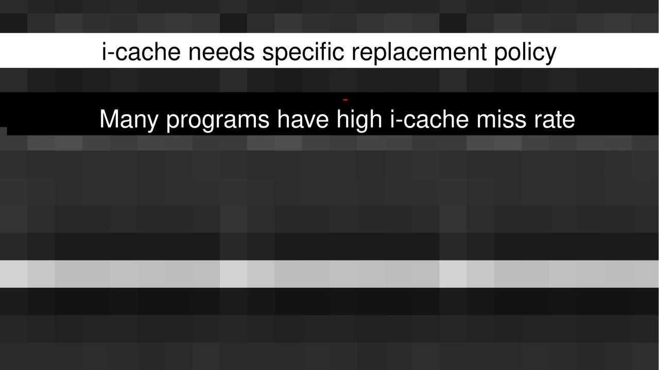
ISCA 2018 lightning talk slide 3: Instruction-cache motivation. The slide highlights high instruction-cache miss rates across programs.
03
Instruction-cache motivation

The slide highlights high instruction-cache miss rates across programs.

Open slide at full size ↗
ISCA 2018 lightning talk slide 4: Prior dead-block prediction. A data-cache technique motivates the new policy while leaving front-end behavior unresolved.
04
Prior dead-block prediction

A data-cache technique motivates the new policy while leaving front-end behavior unresolved.

Open slide at full size ↗
ISCA 2018 lightning talk slide 5: ISCA session and results. The final slide identifies the presentation session and compares the policies.
05
ISCA session and results

The final slide identifies the presentation session and compares the policies.

Open slide at full size ↗

Figures are reproduced from the linked papers. Results refer to the models, workloads, hardware, and experimental conditions evaluated in each study.

Research areas

Microarchitecture & security

Discovering how hidden processor behavior exposes information, and developing hardware defenses that learn from execution.

Side channels · Reverse engineering · Adaptive defenses

Secure AI accelerators

Investigating the security consequences of performance optimizations in on-chip accelerators, including data-dependent timing, sparsity, and power gating.

Accelerator security · AI privacy · Hardware measurement

AI for computer architecture

Developing compact learning mechanisms and tools that help architects explain hardware behavior and improve processor performance.

Learning-based prediction · Cache systems · Generative AI

Research artifacts

Code, setup instructions, and citations. Cite the paper and the exact software version used in your work.

ASPLOS 2026

CacheMind

No archived software release DOI has been verified. Cite the paper and record the exact Git commit used.

Installation and requirements

The repository supplies a Linux Conda environment with Python 3.8.20 and CUDA 12.1 dependencies. Remove the machine-specific prefix before creating a local environment.

git clone https://github.com/kaushal1803/cachemind.git
cd cachemind
sed '/^prefix:/d' code_files/RAG.yaml > RAG-local.yaml
conda env create -n cachemind -f RAG-local.yaml
conda activate cachemind

The public checkout includes notebooks and benchmark questions, but omits the trace data, prepared dataset, and local model checkpoints referenced by the notebooks. Follow the installation guide to prepare inputs, choose a backend, and align notebook paths. The historical environment may need package updates.

MICRO 2025

GateBleed

Archived artifact · September 1, 2025
Software DOI: 10.5281/zenodo.17019733 · Zenodo release archive

This preserved snapshot predates the current repository. Cite its software DOI when using the archived artifact; the paper has a separate DOI.

Installation and requirements

Requires an Intel AMX-capable system. The repository reports testing on dual-socket Intel Xeon Gold 5420+ (Sapphire Rapids), with RHEL 9.4 and Ubuntu 22.04.

git clone https://github.com/jkalya/gatebleed.git
cd gatebleed
python3 -m venv .venv
. .venv/bin/activate
python -m pip install -r requirements.txt

Each experiment includes its own README and build instructions. See the installation guide for the first performance-stage experiment, dependencies, and archived-version details.